Downloaded 10 times

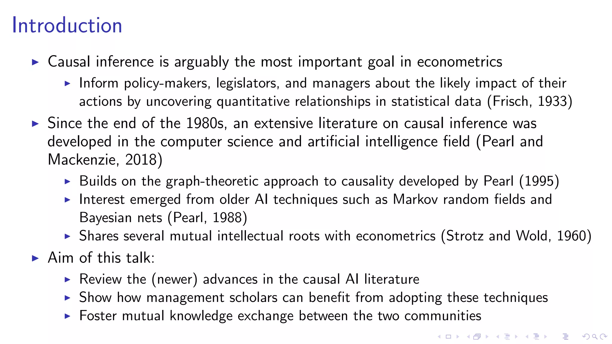


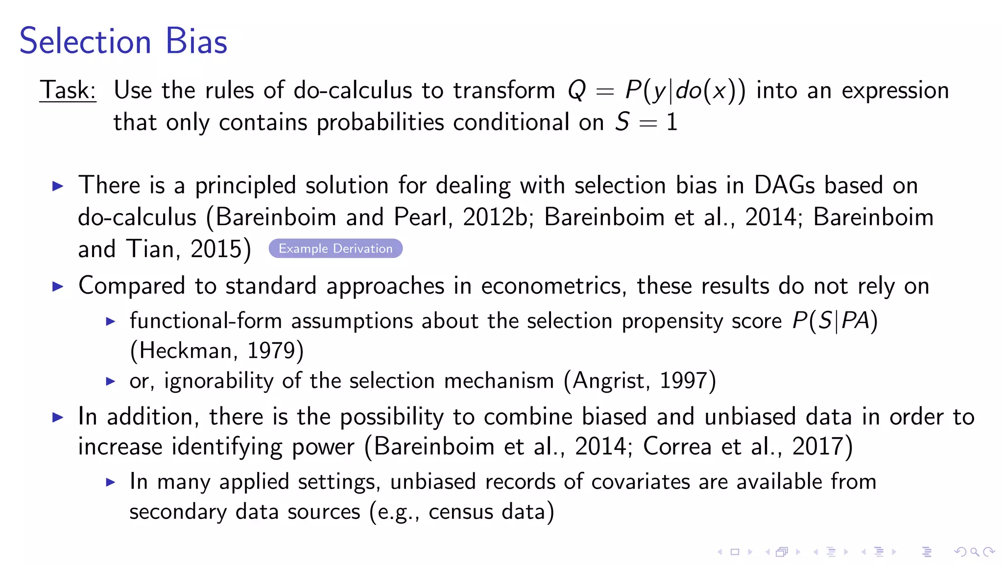
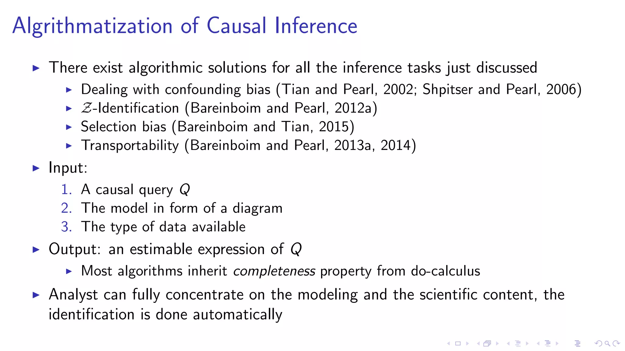
![Colliders – R example
# Create two independent normally d i s t r i b u t e d v a r i a b l e s
x <− rnorm (1000)
y <− rnorm (1000)
# Construct z as being equal to one i f x + y > 0 , and zero
otherwise
z <− 1∗ ( x + y > 0)
# By design , there i s no c o r r e l a t i o n between x and y
cor ( x , y )
# But i f we c o n d i t i o n on z==1, we f i n d a ne gati ve c o r r e l a t i o n
cor ( x [ z==1], y [ z==1])](https://image.slidesharecdn.com/hunermund-causalinferenceinmlandai-200508131351/75/Hunermund-causal-inference-in-ml-and-ai-17-2048.jpg)
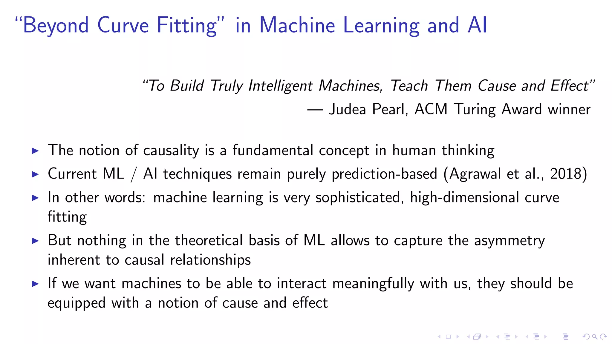
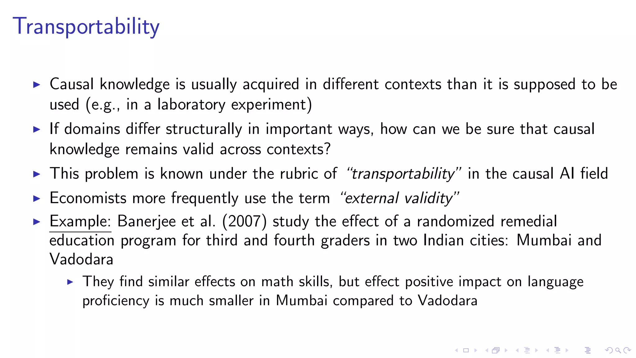
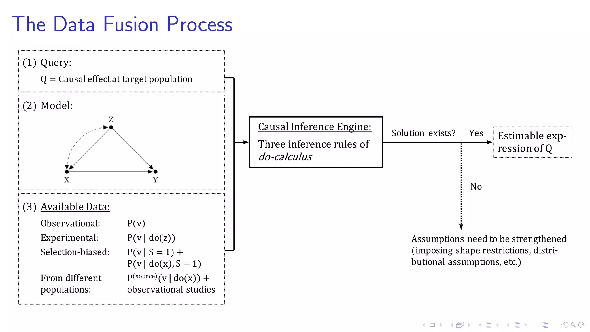
![“Correlation doesn’t imply causation” – R example
# Create background f a c t o r s f o r nodes
e x <− rnorm (10000)
e y <− rnorm (10000)
e z <− rnorm (10000)
# Create nodes f o r the DAG: y <− x , y <− z , x <− z
z <− 1∗ ( e z > 0)
x <− 1∗ ( z + e x > 0.5)
y <− 1∗ ( x + z + e y > 2)
y dox <− 1∗ (1 + z + e y > 2)
# We see that P( y | do ( x=1)) i s not equal to P( y | x=1)
mean( y dox )
mean( y [ x==1])](https://image.slidesharecdn.com/hunermund-causalinferenceinmlandai-200508131351/75/Hunermund-causal-inference-in-ml-and-ai-21-2048.jpg)
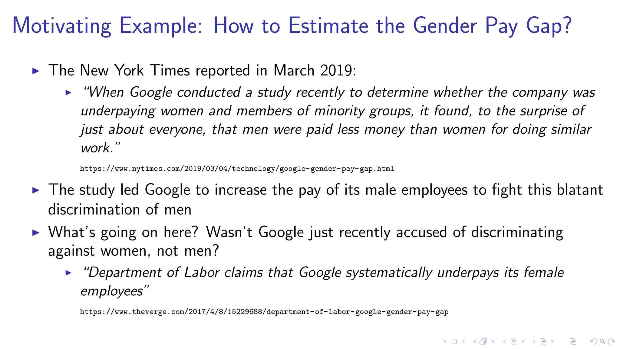
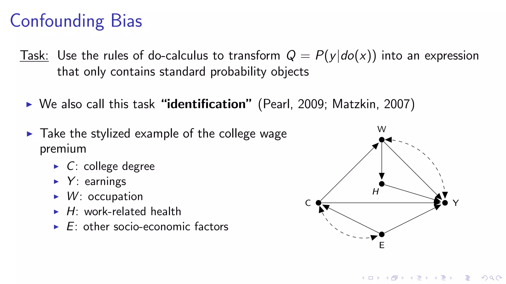
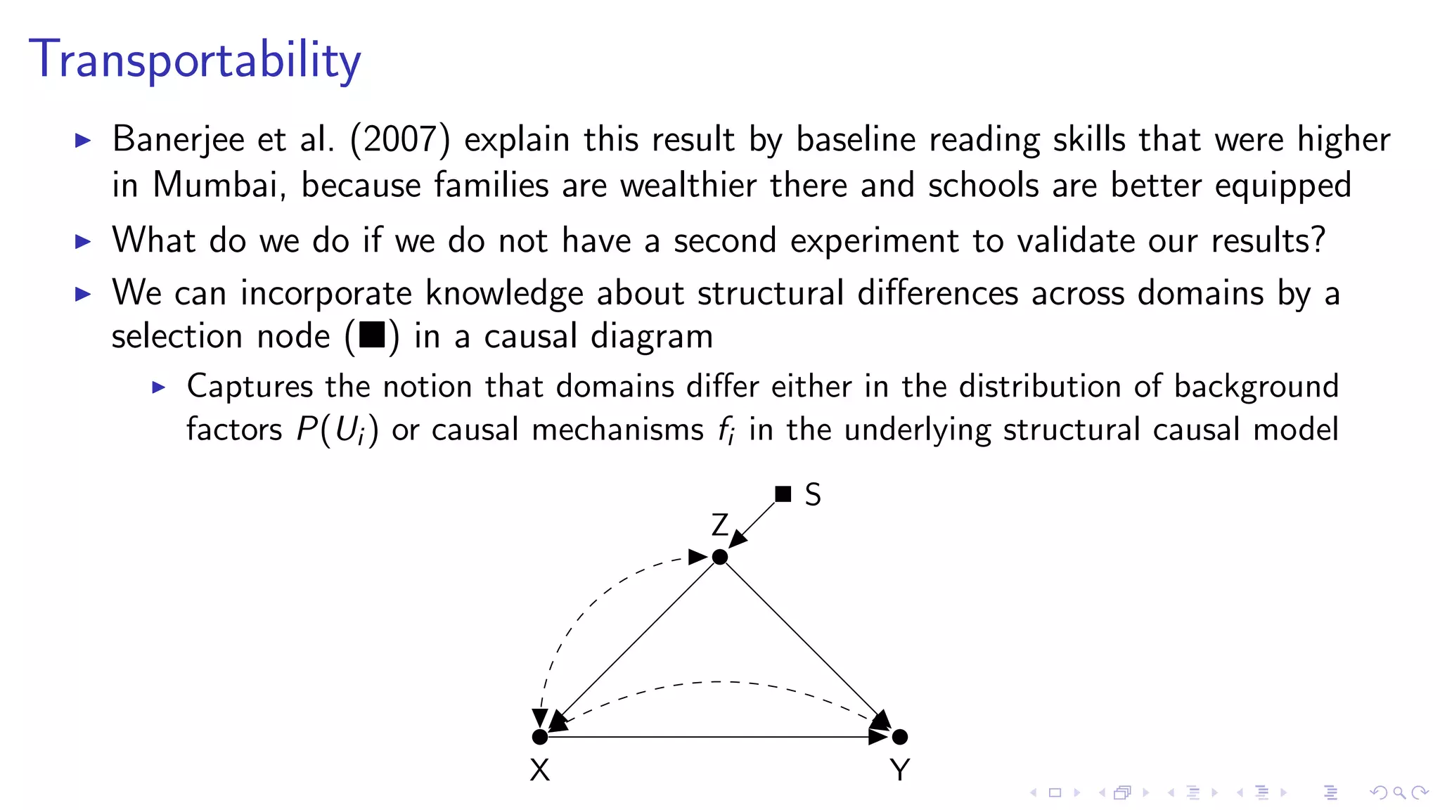
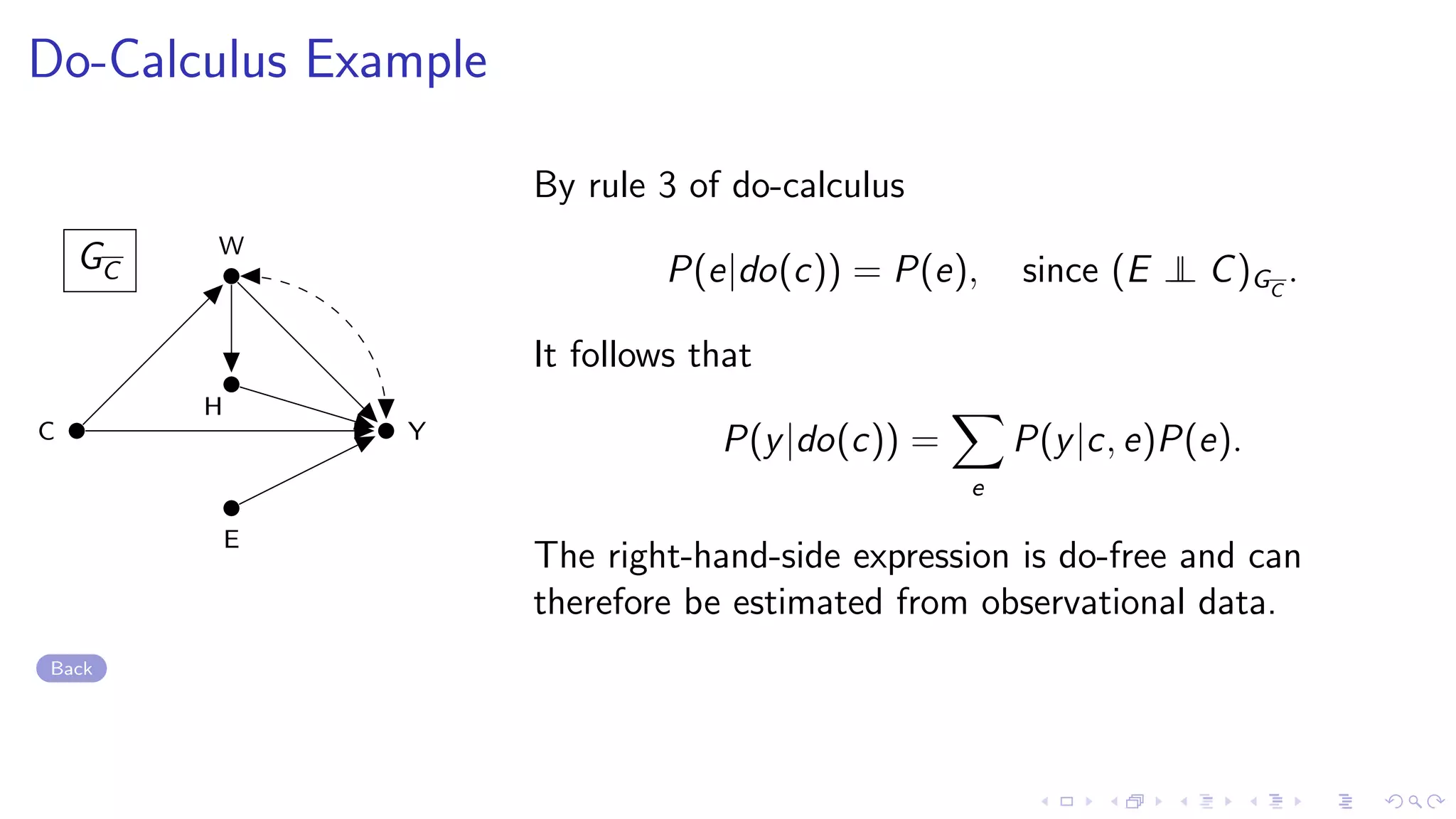
![Do-Calculus
Theorem: Rules of do Calculus (Pearl, 2009, p. 85)
Let G be the directed acyclic graph associated with a [structural] causal model [...], and let P(·) stand
for the probability distribution induced by that model. For any disjoint subset of variables X, Y , Z,
and W , we have the following rules.
Rule 1 (Insertion/deletion of observations):
P(y|do(x), z, w) = P(y|do(x), w) if (Y ⊥⊥ Z|X, W )GX
.
Rule 2 (Action/observation exchange): Illustration
P(y|do(x), do(z), w) = P(y|do(x), z, w) if (Y ⊥⊥ Z|X, W )GXZ
.
Rule 3 (Insertion/deletion of actions):
P(y|do(x), do(z), w) = P(y|do(x), w) if (Y ⊥⊥ Z|X, W )GXZ(W )
,
where Z(W ) is the set of Z-nodes that are not ancestors of any W -node in GX .](https://image.slidesharecdn.com/hunermund-causalinferenceinmlandai-200508131351/75/Hunermund-causal-inference-in-ml-and-ai-22-2048.jpg)

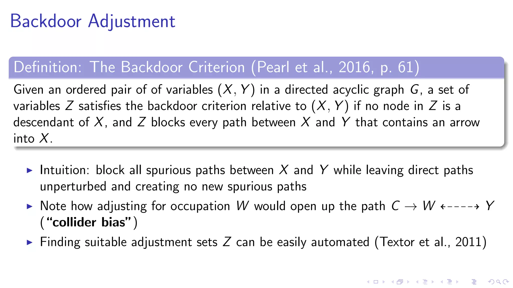
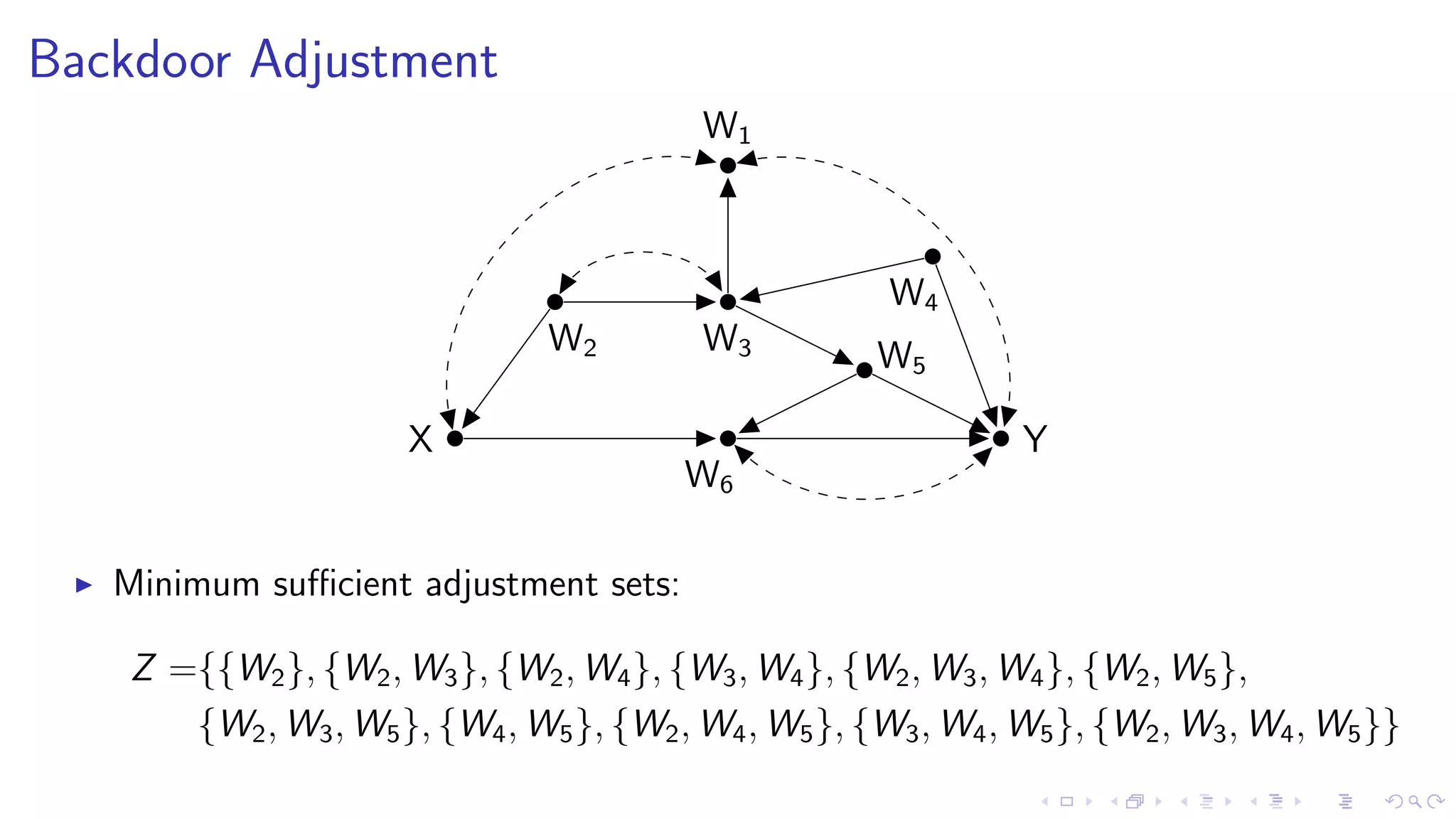
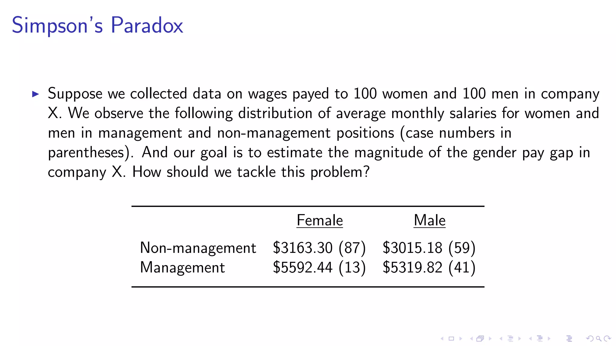
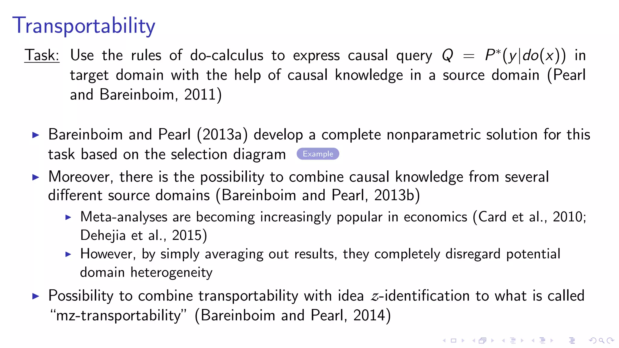
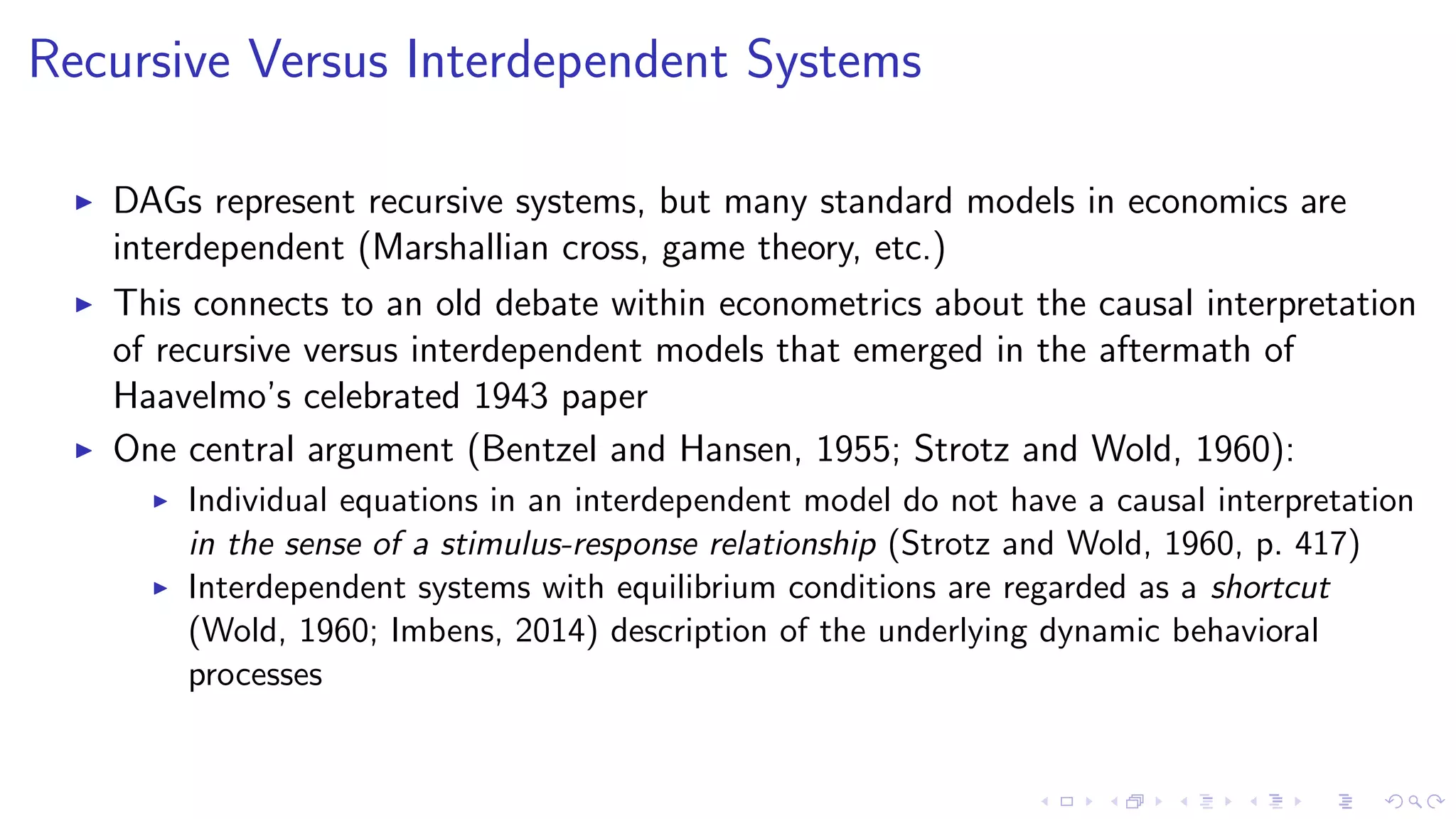
![Backdoor Adjustment – R example
# Define DGP as in p r e v i o u s R example
# Adjustment formula : P( y | do ( x=1)) = P( y | x=1, z=1)∗P( z=1) + P( y | x
=1, z=0)∗P( z=0)
mean( y [ x==1 & z==1]) ∗ mean( z==1) + mean( y [ x==1 & z==0]) ∗ mean( z
==0)
# Estimation v i a i n v e r s e p r o b a b i l i t y weighting
df <− df %>% group by ( z ) %>% mutate ( weight = mean( x ) )
weight <− df $ weight
y weighted <− y / weight](https://image.slidesharecdn.com/hunermund-causalinferenceinmlandai-200508131351/75/Hunermund-causal-inference-in-ml-and-ai-30-2048.jpg)
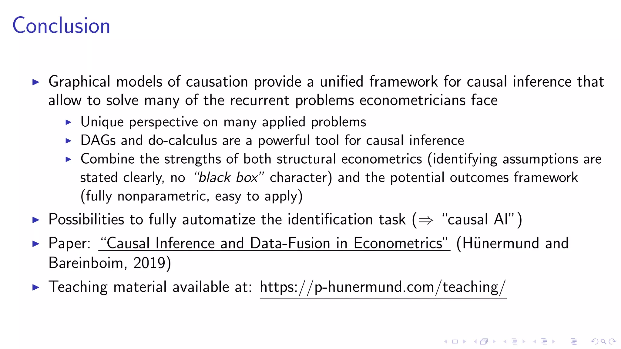


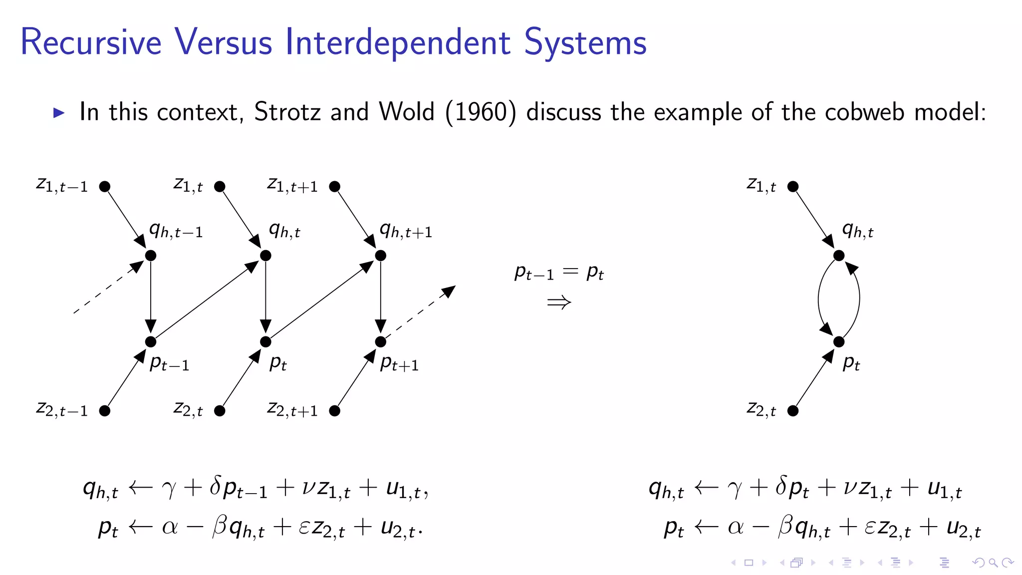
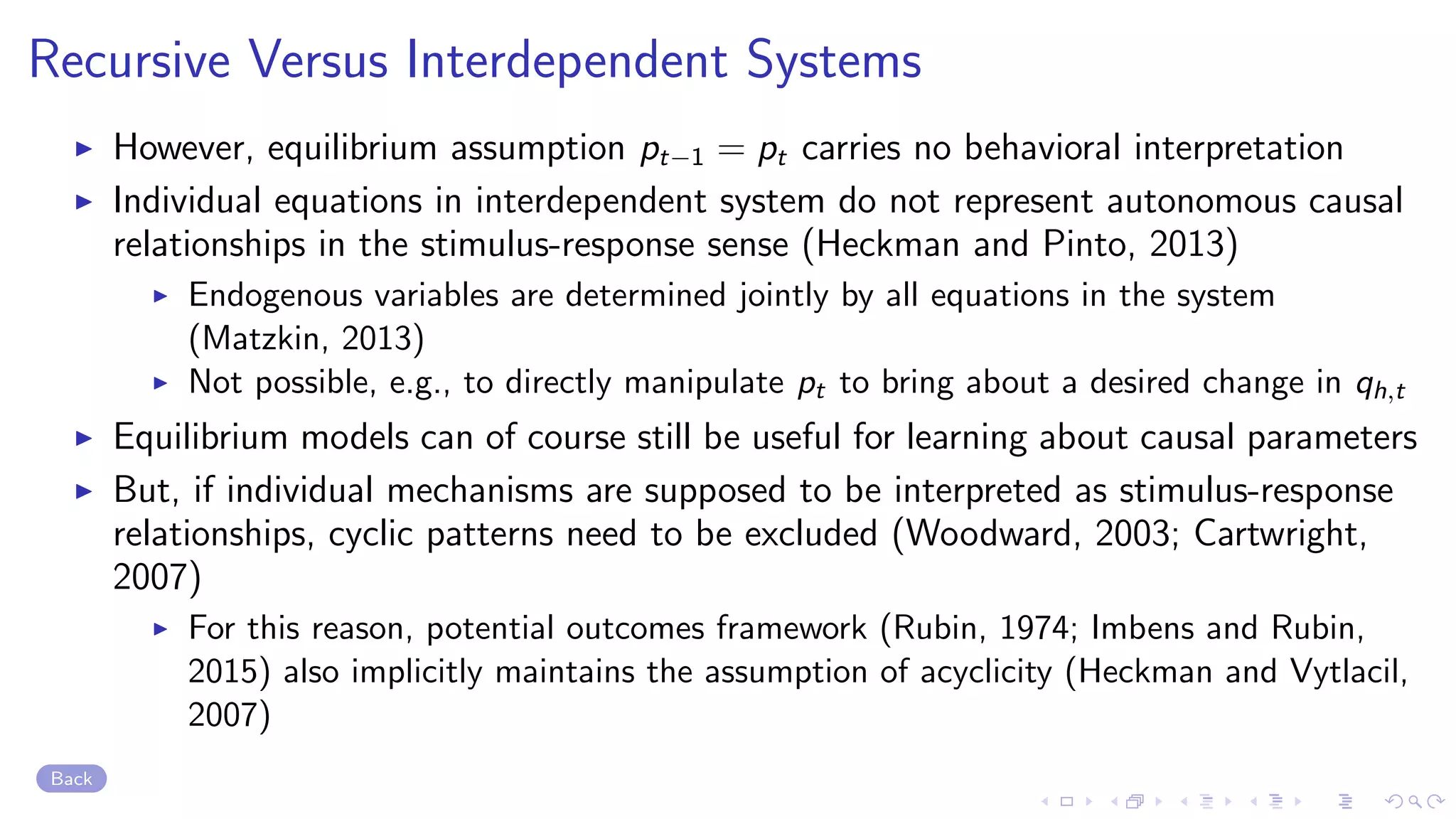
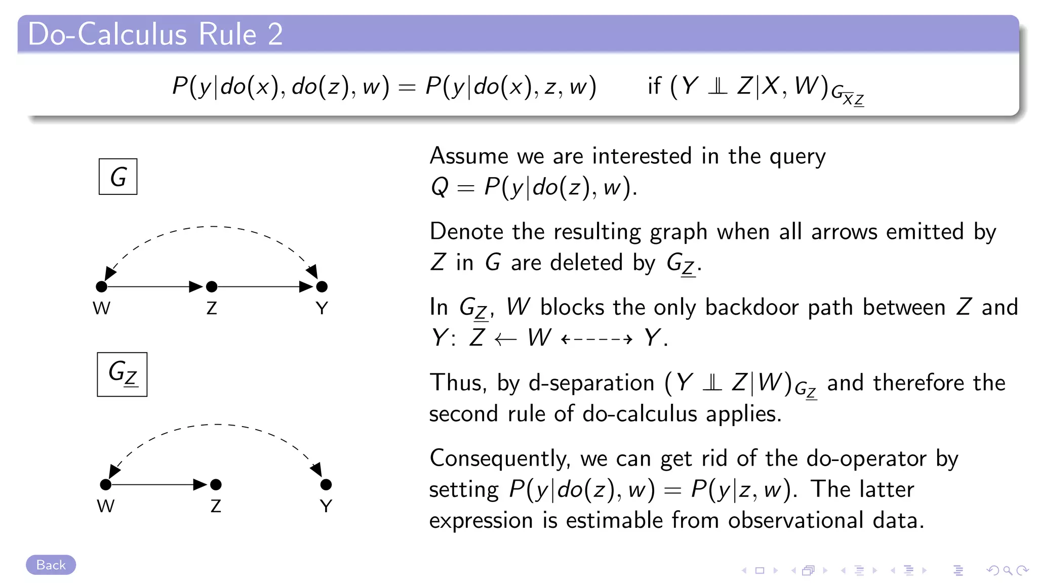
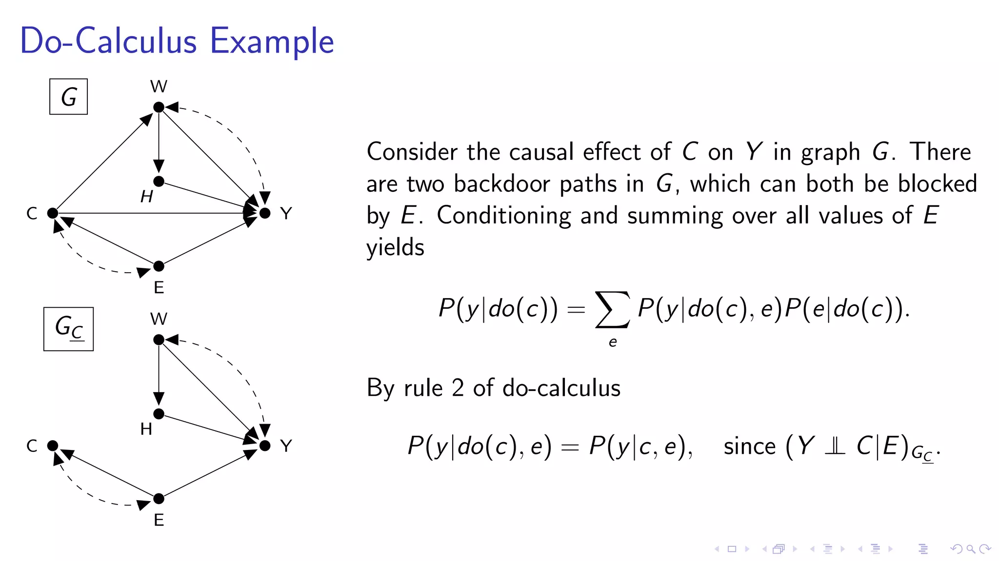
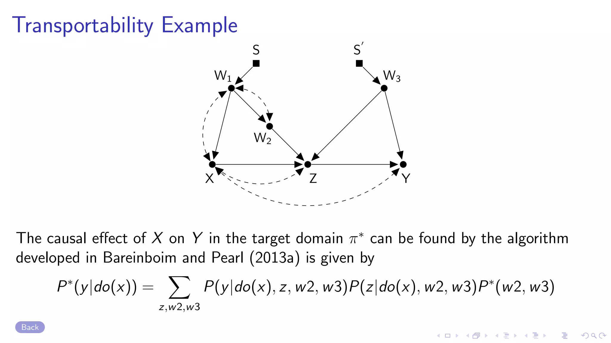

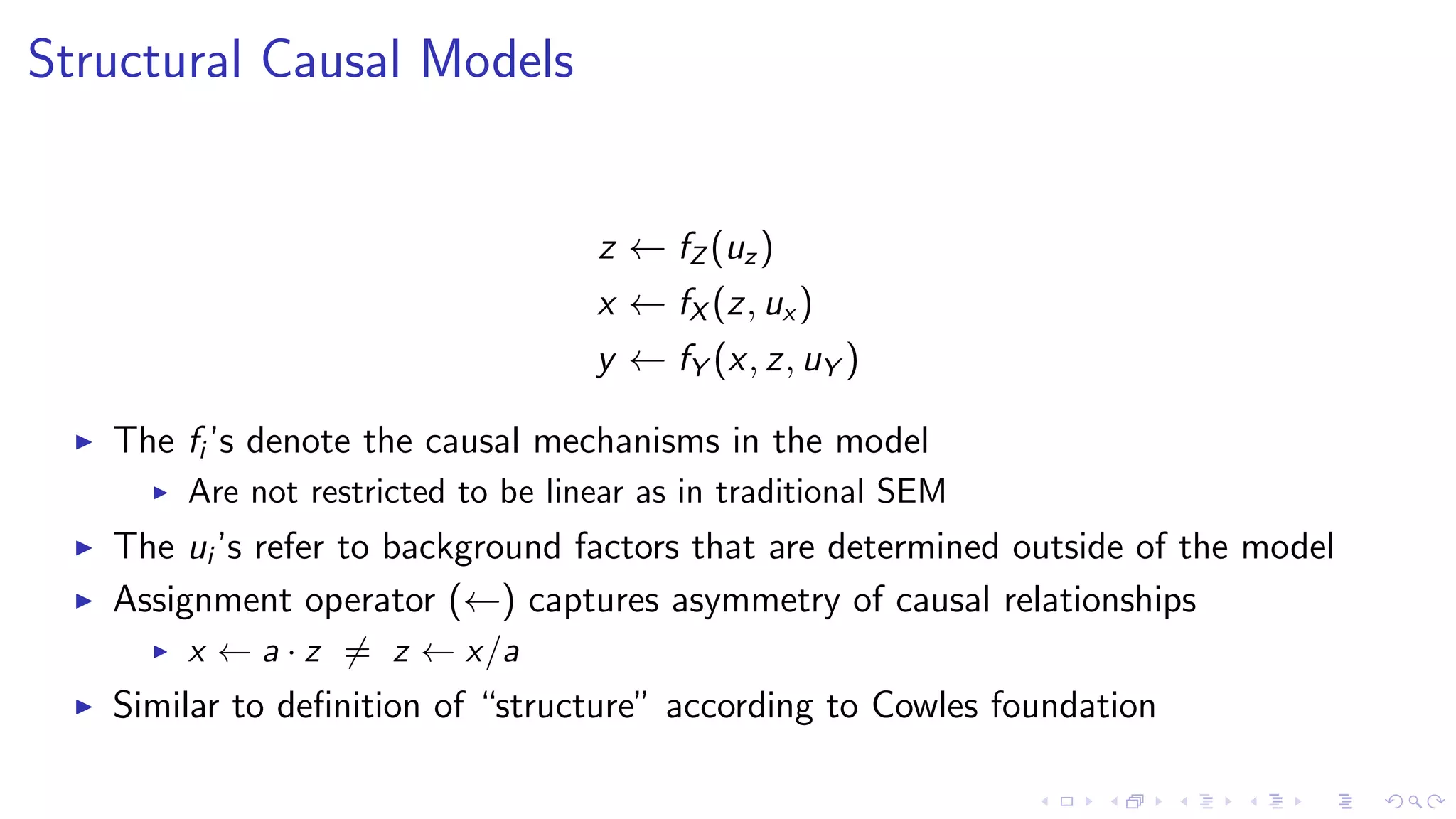
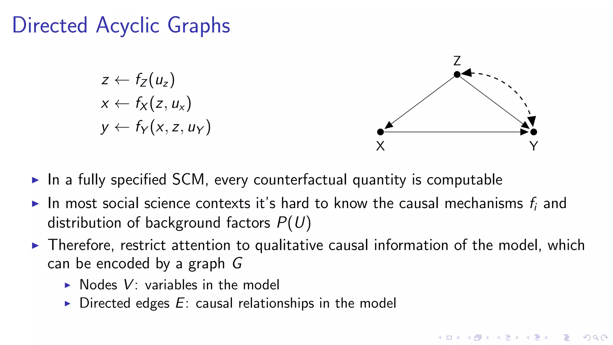
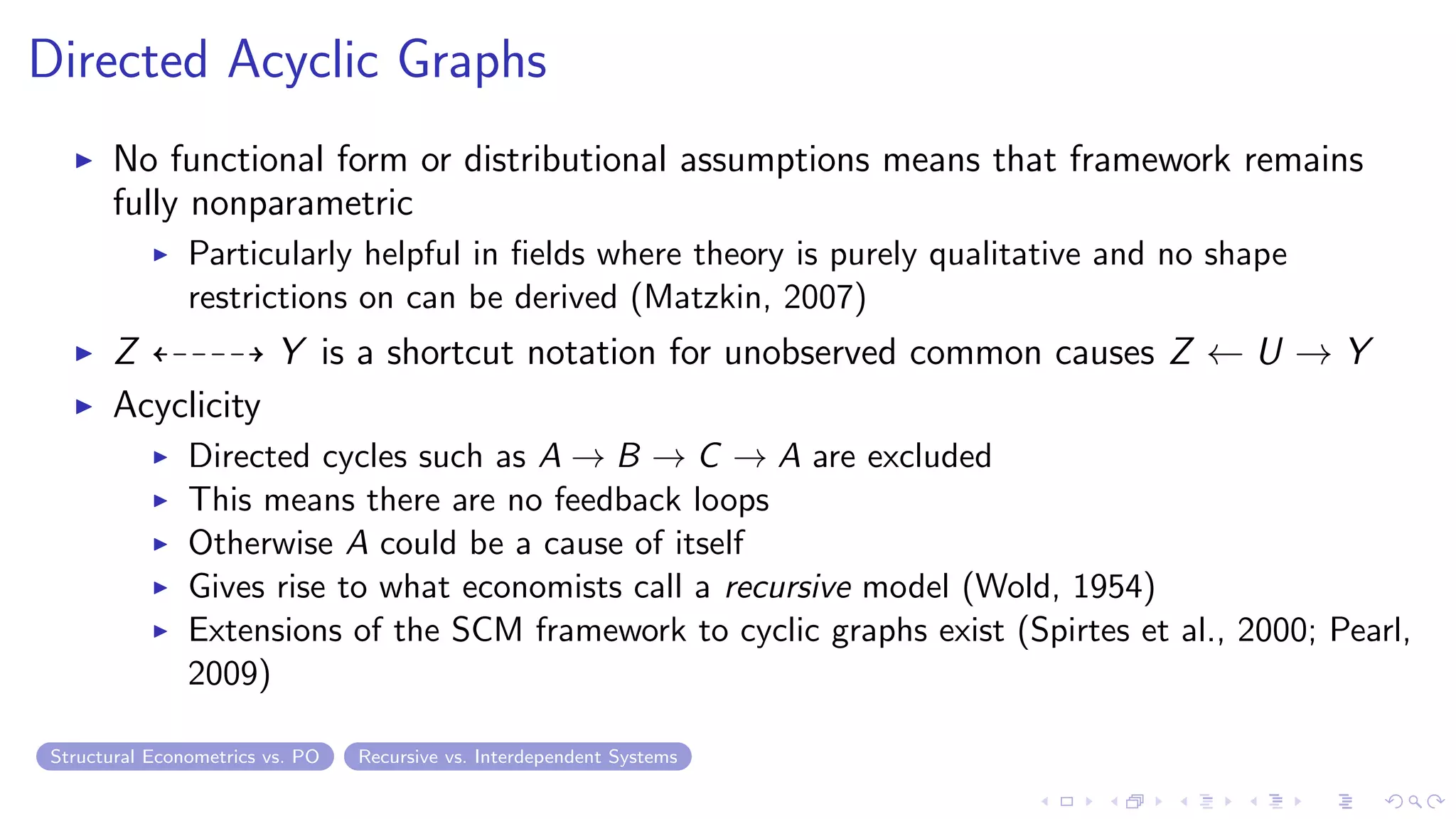
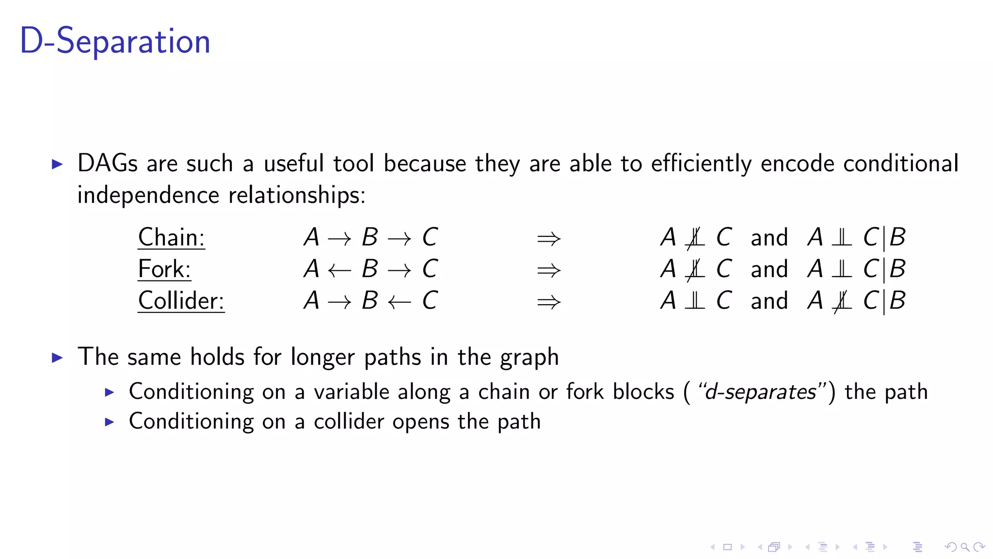
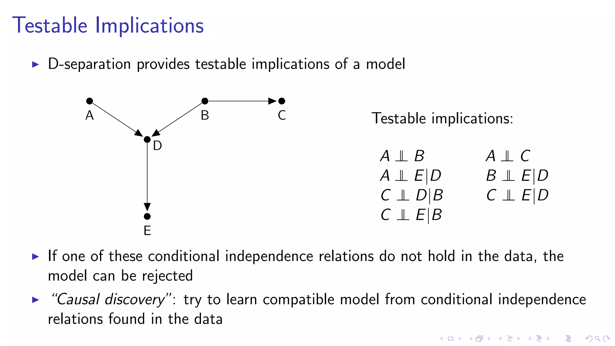
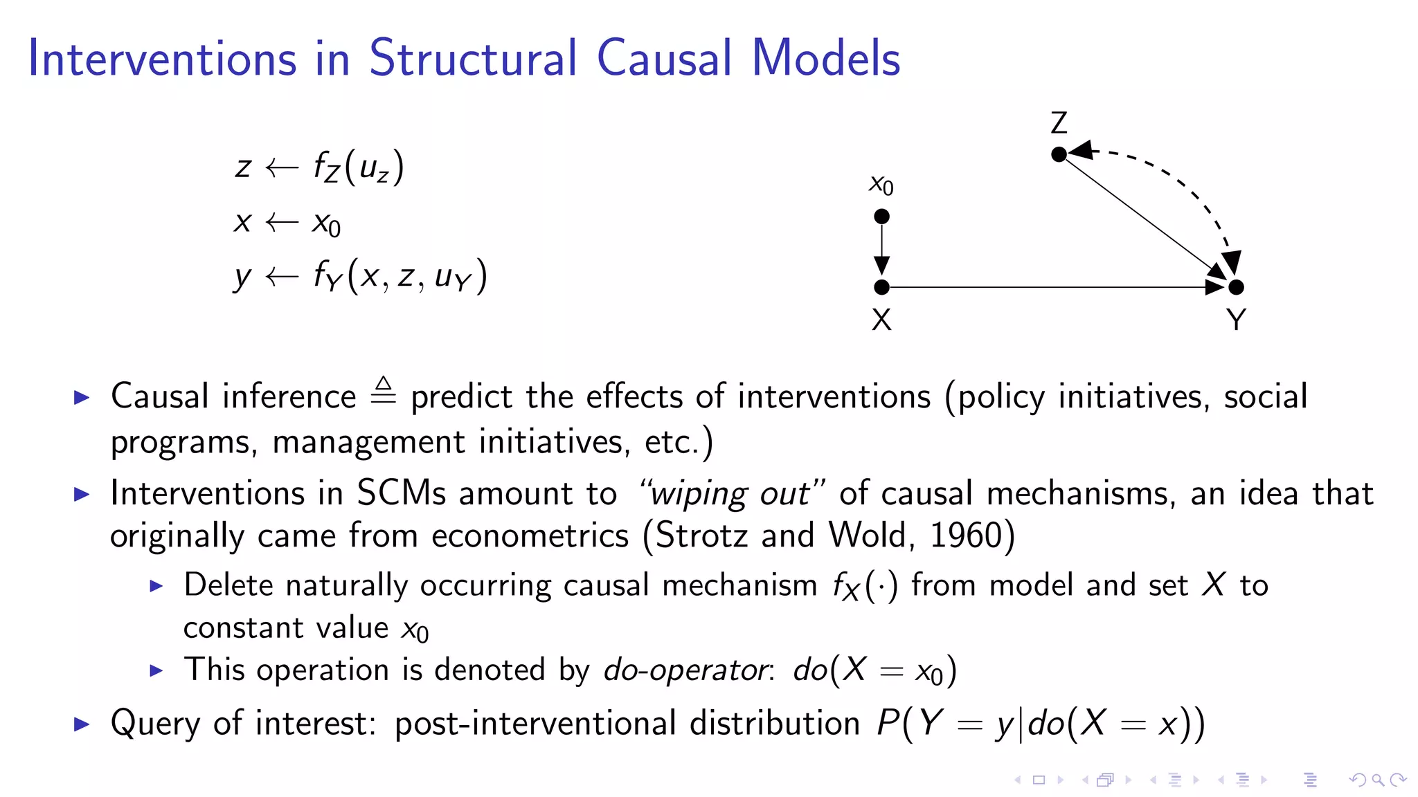
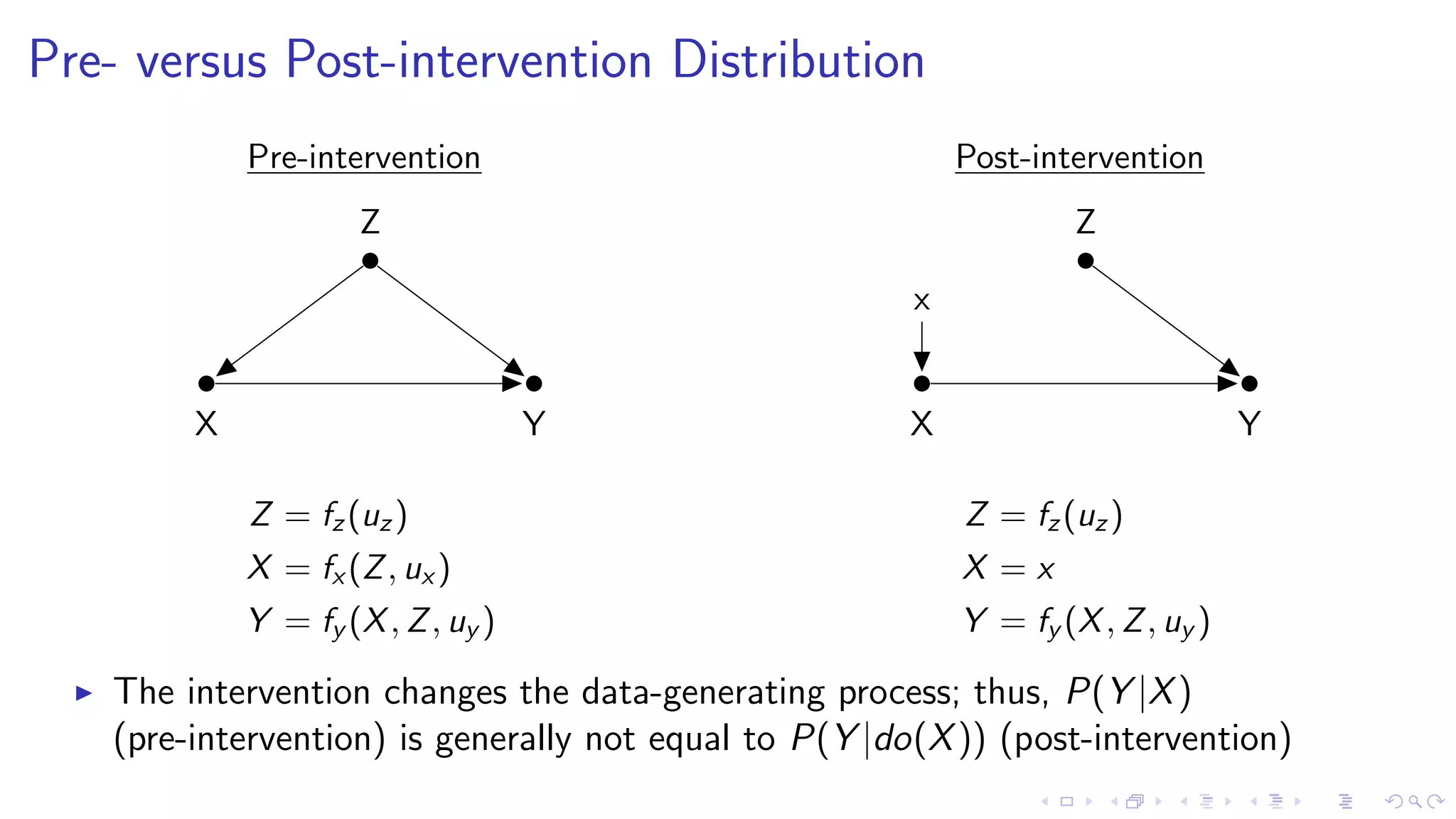
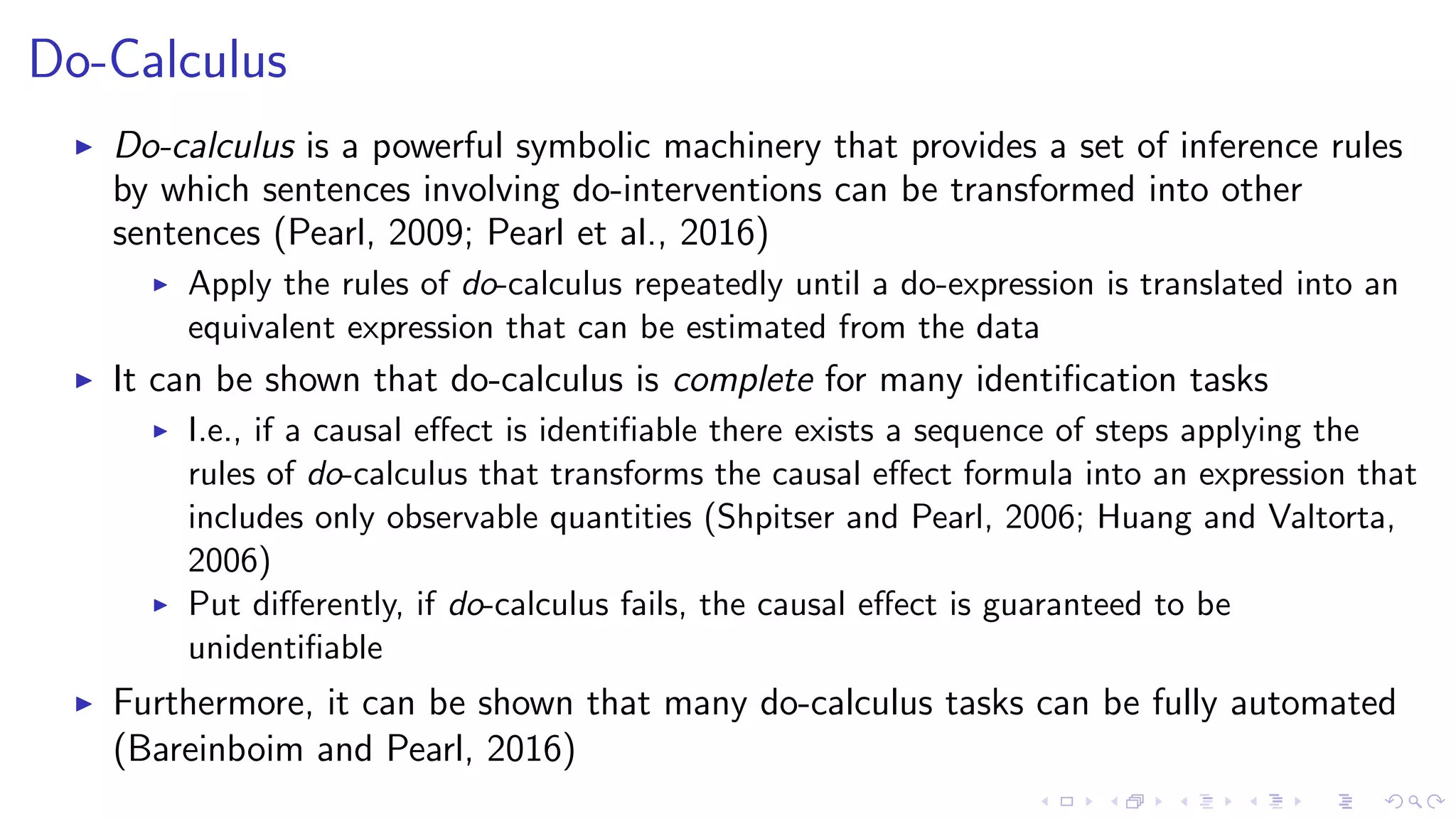
1. The document discusses causal inference in machine learning and artificial intelligence, focusing on recent advances in the causal AI literature and how management scholars can benefit from adopting these techniques. 2. It reviews the concept of structural causal models and directed acyclic graphs which are used to encode causal relationships and infer how interventions such as policies can affect outcomes. 3. The document also discusses do-calculus, a set of rules for deriving the effects of interventions from observational data using conditional independencies encoded in a causal graph.


![Vibe Coding vs. Spec-Driven Development [Free Meetup]](https://cdn.slidesharecdn.com/ss_thumbnails/vibecodingvsspecdrivendevelopment-251209105622-43f455e7-thumbnail.jpg?width=640&height=640&fit=bounds)


