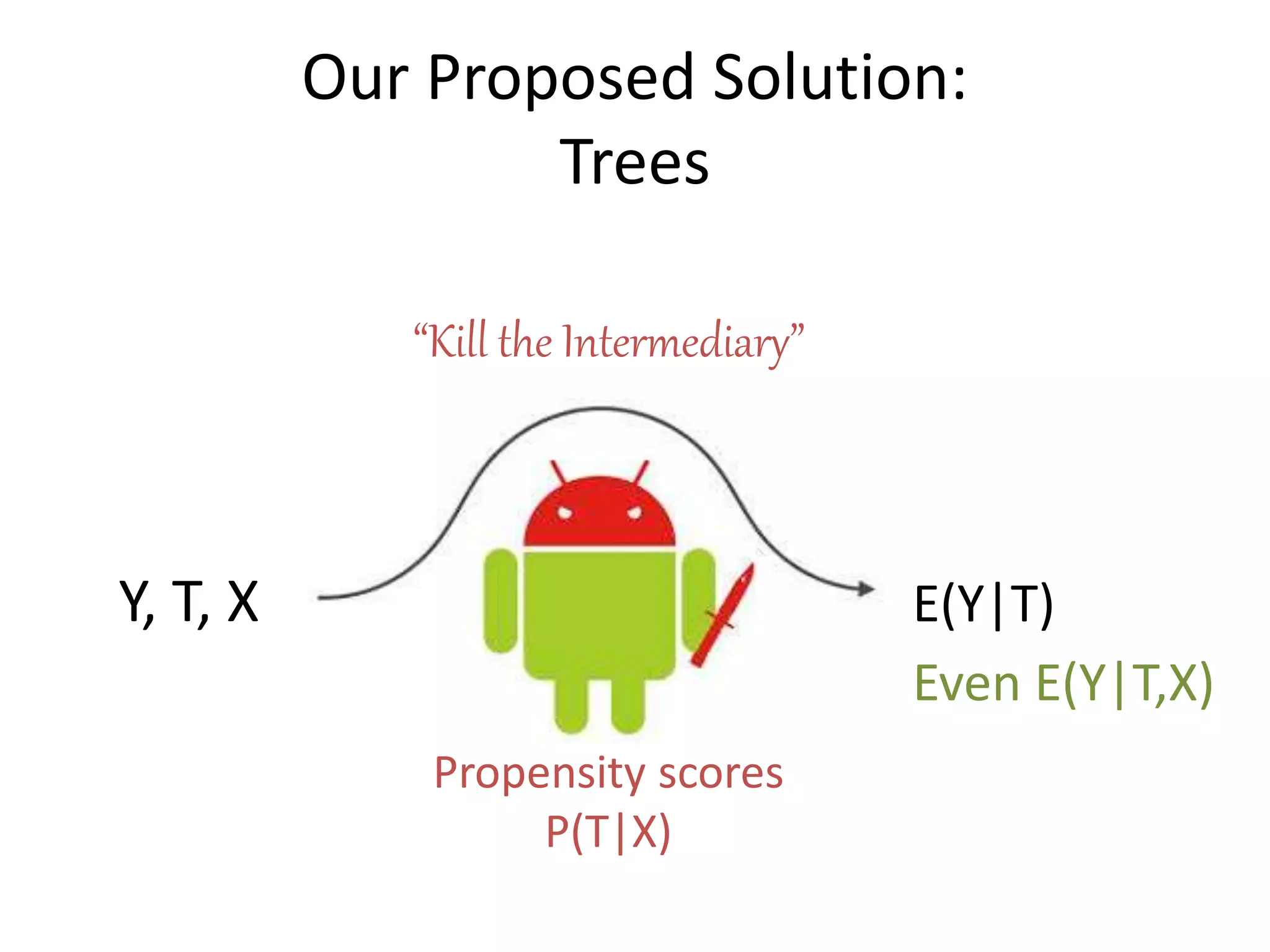
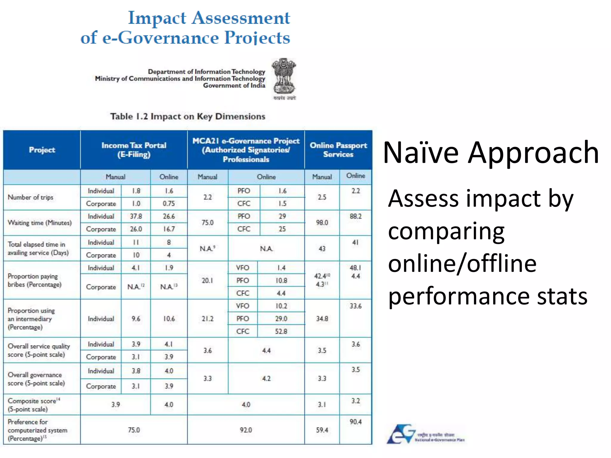
Download to read offline

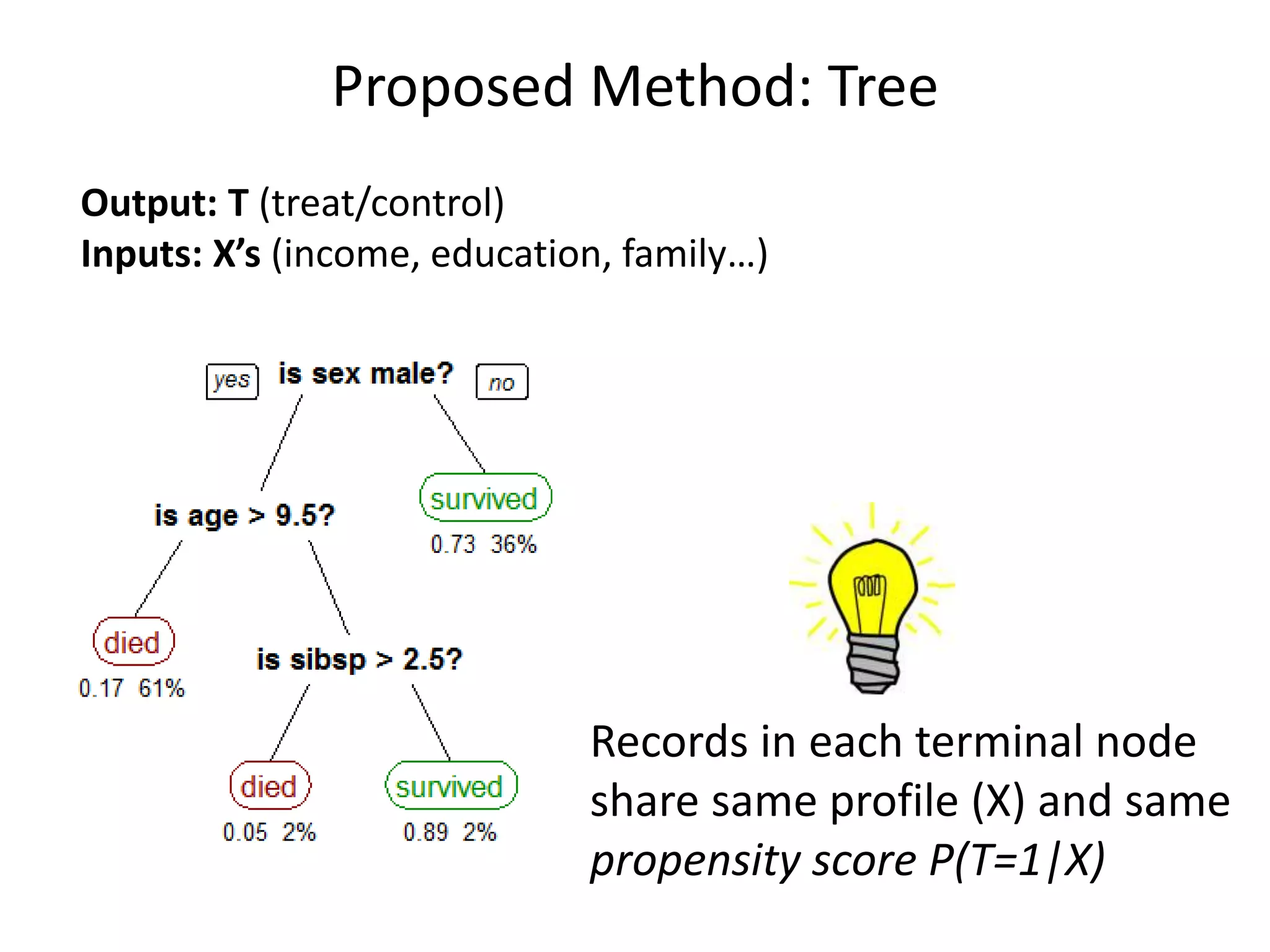
![Tree-Based Approach
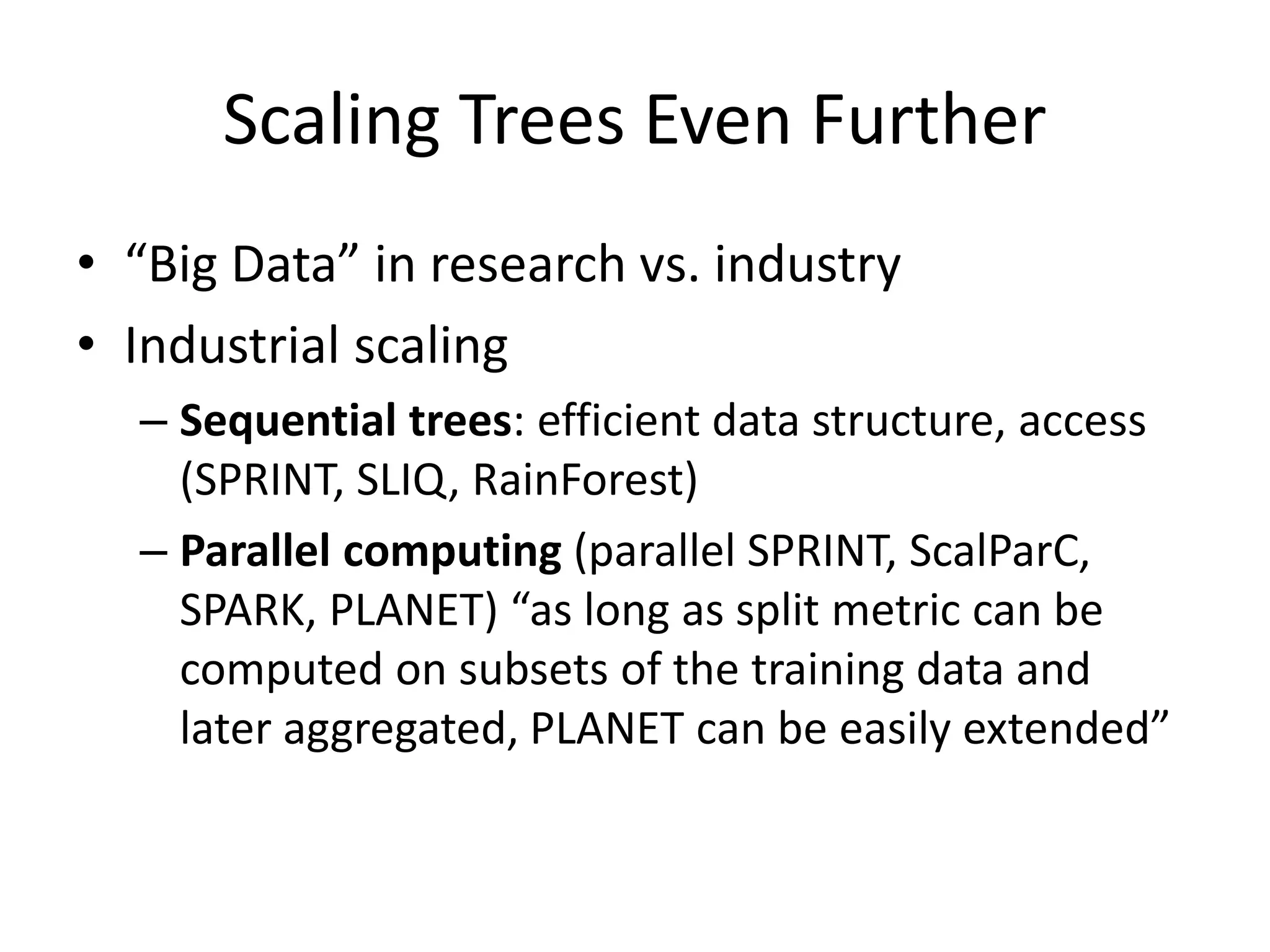
Four steps:
1. Run selection model: fit tree T = f(X)
2. Visualize tree; see unbalanced X’s
3. Treat each terminal node as sub-sample;
conduct terminal-node-level performance
analysis
4. Present terminal-node-analyses visually
5. [optional]: combine analyses from nodes with
homogeneous effects
Like PS, assumes observable self-selection](https://image.slidesharecdn.com/treesforcausalresearchwombatmonashnov2019-191129032230/75/Repurposing-Classification-Regression-Trees-for-Causal-Research-with-High-Dimensional-Data-12-2048.jpg)
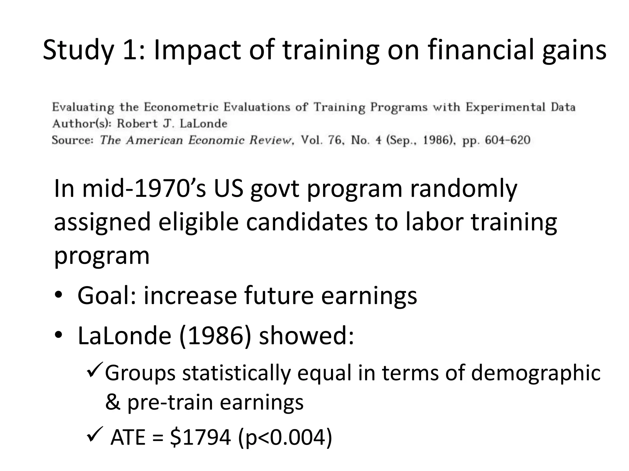
![Labor Training effect:
Observational control group
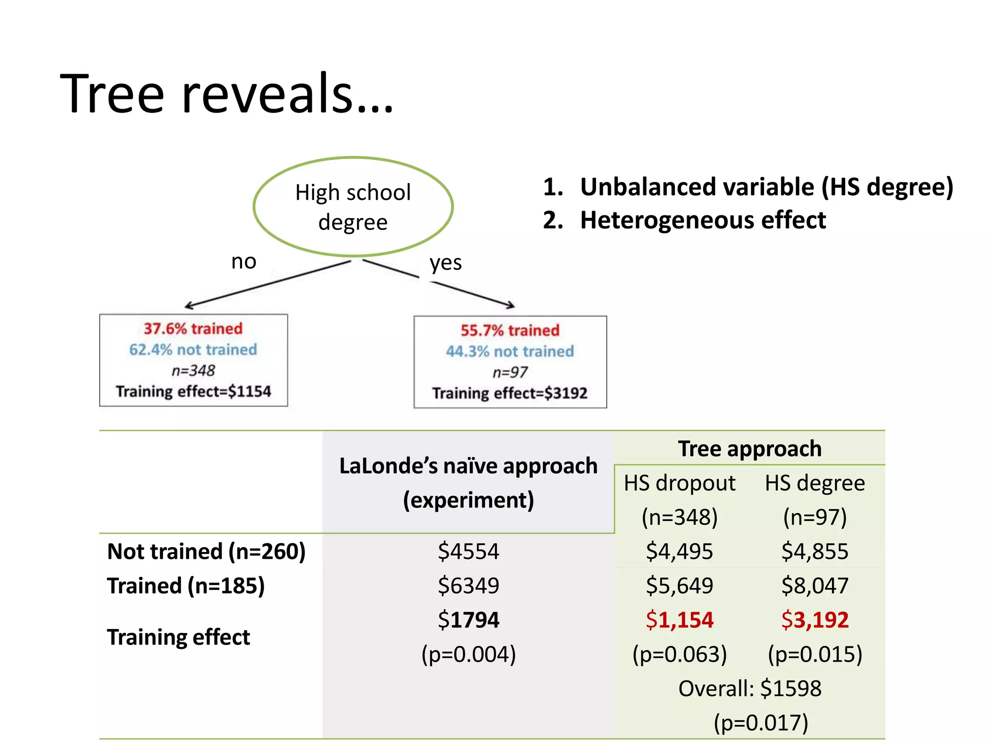
• LaLonde also compared with observational
control groups (PSID, CPS)
– experimental training group vs. obs control
– showed training effect not estimated correctly with
structural equations
• Dehejia & Wahba (1999,2002) re-analyzed CPS
control group (n=15,991), using PSM
– Effects in range [$1122, $1681], depends on settings
– “Best” setting effect: $1360
– Uses only 119 control group members (out of 15,991)](https://image.slidesharecdn.com/treesforcausalresearchwombatmonashnov2019-191129032230/75/Repurposing-Classification-Regression-Trees-for-Causal-Research-with-High-Dimensional-Data-17-2048.jpg)
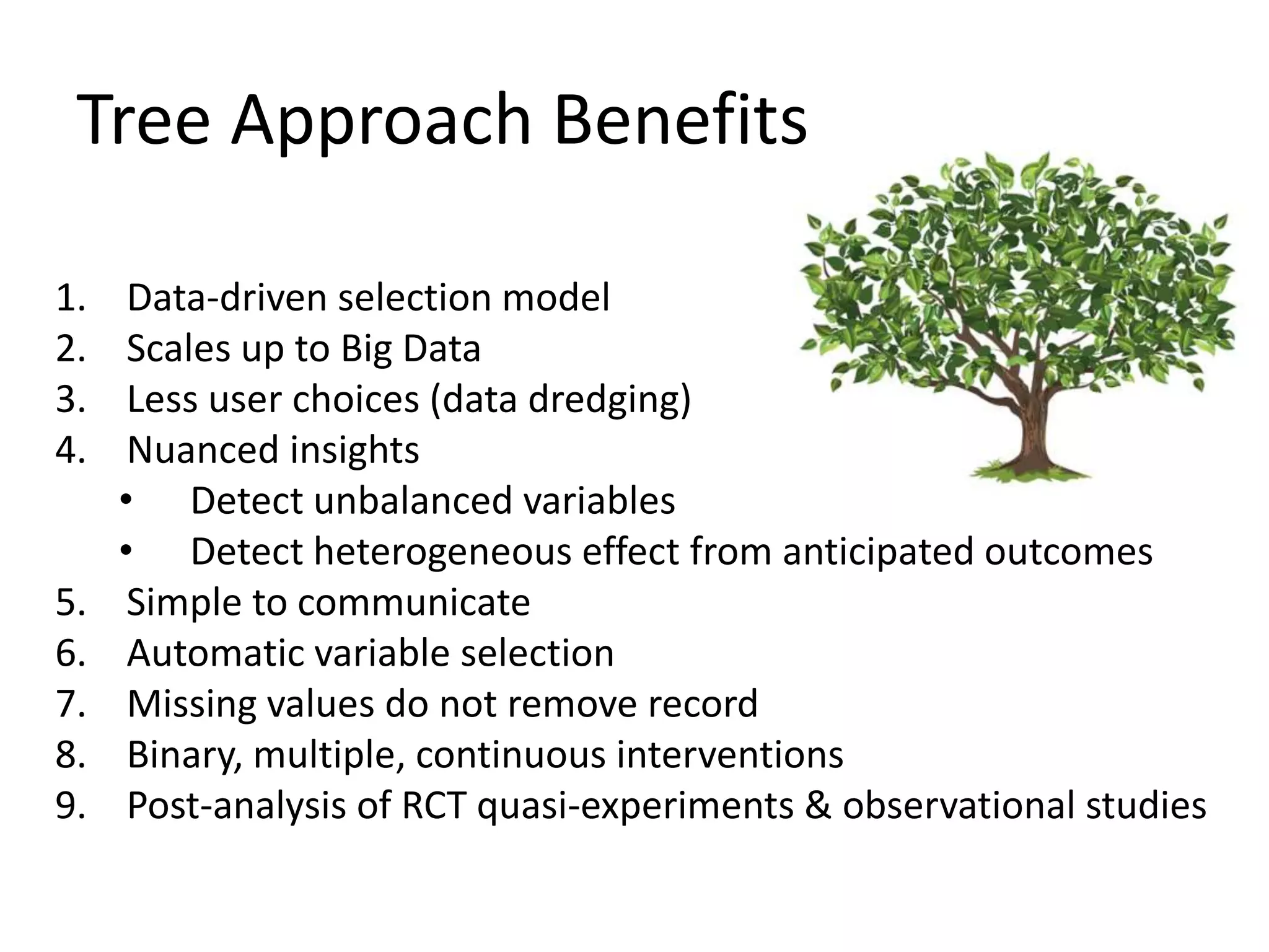
![Tree Approach Limits
1. Assumes selection on observables
2. Need sufficient data
3. Continuous variables can lead to large tree
4. Instability
[possible solution: use variable importance scores (forest)]](https://image.slidesharecdn.com/treesforcausalresearchwombatmonashnov2019-191129032230/75/Repurposing-Classification-Regression-Trees-for-Causal-Research-with-High-Dimensional-Data-30-2048.jpg)
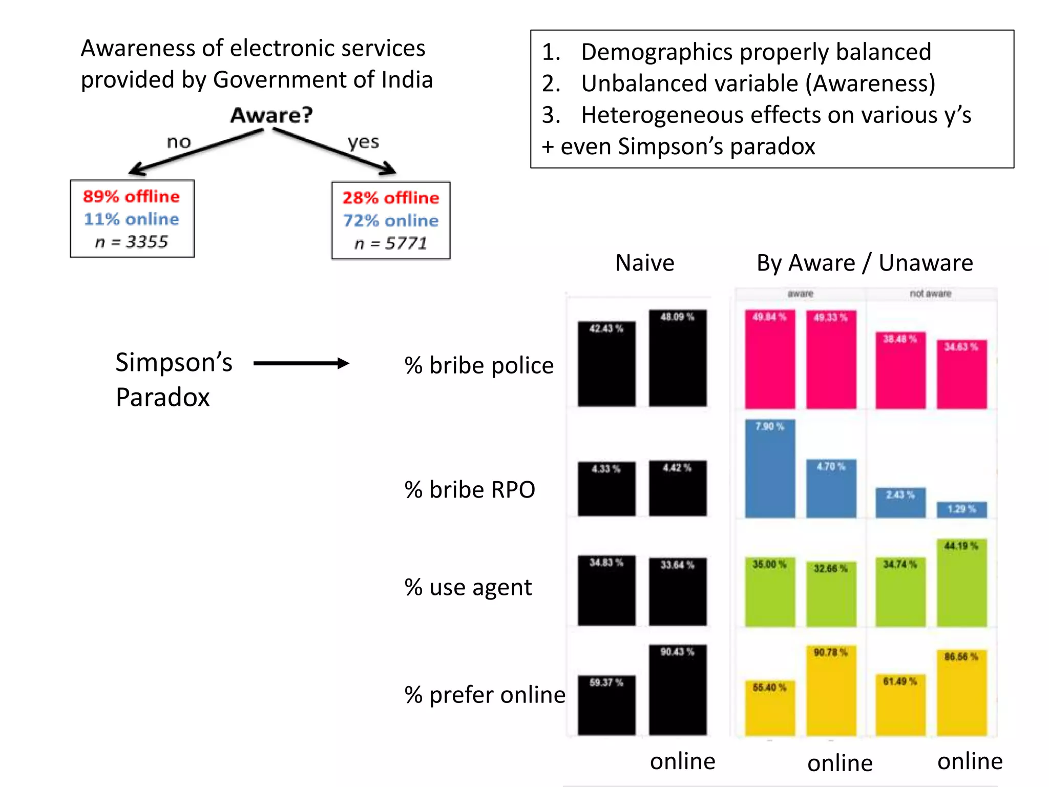
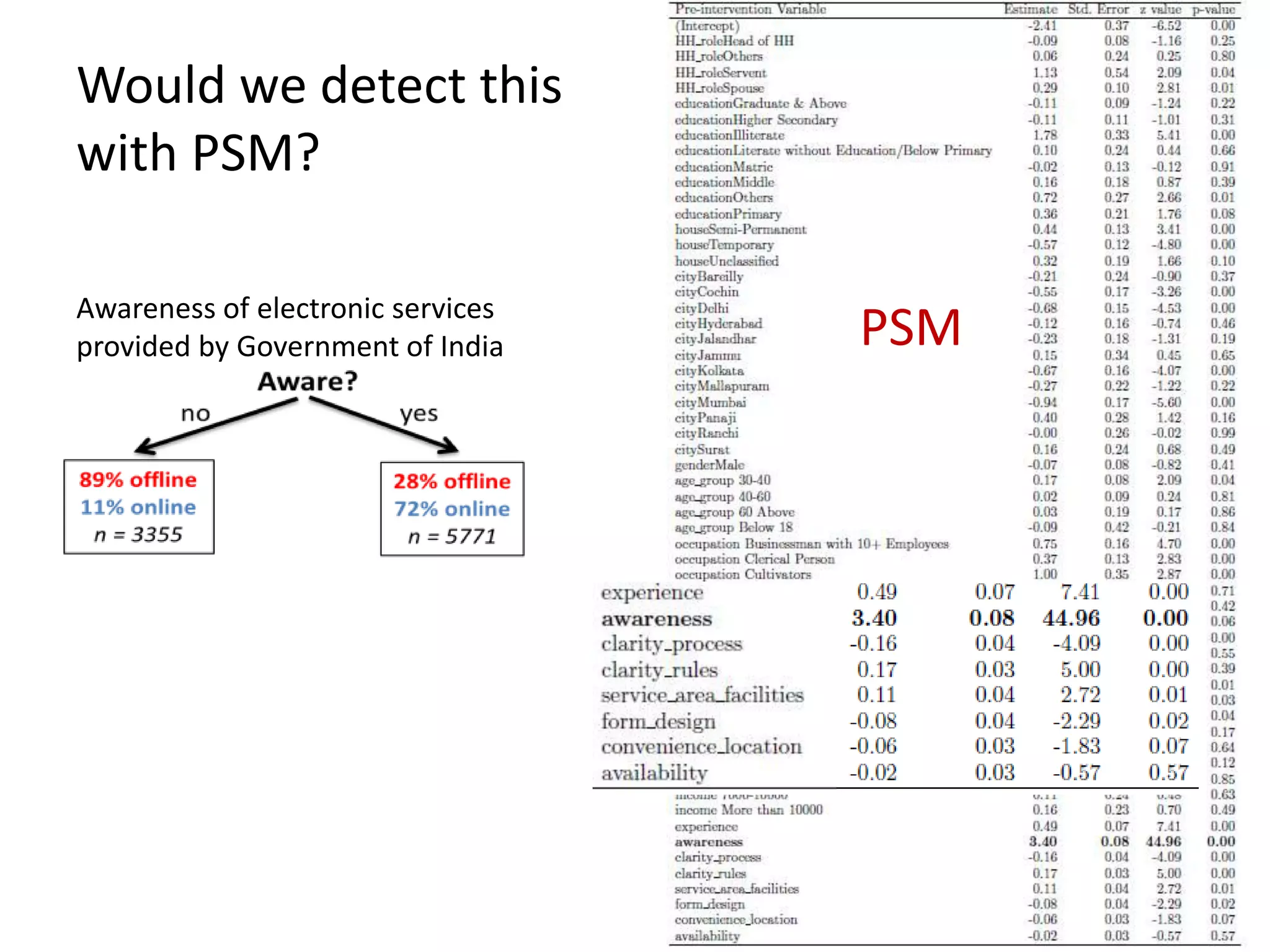
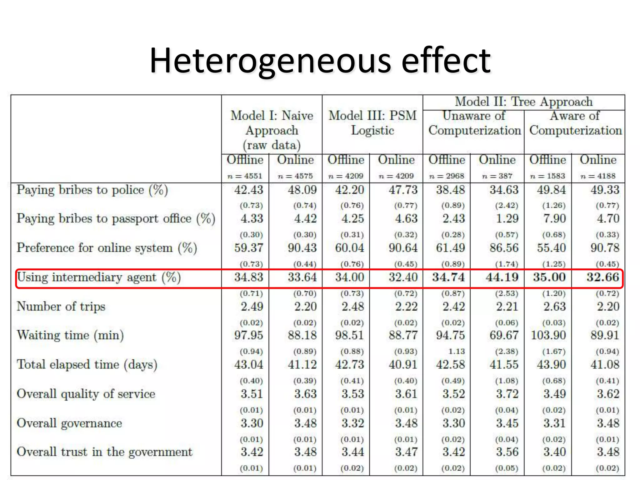
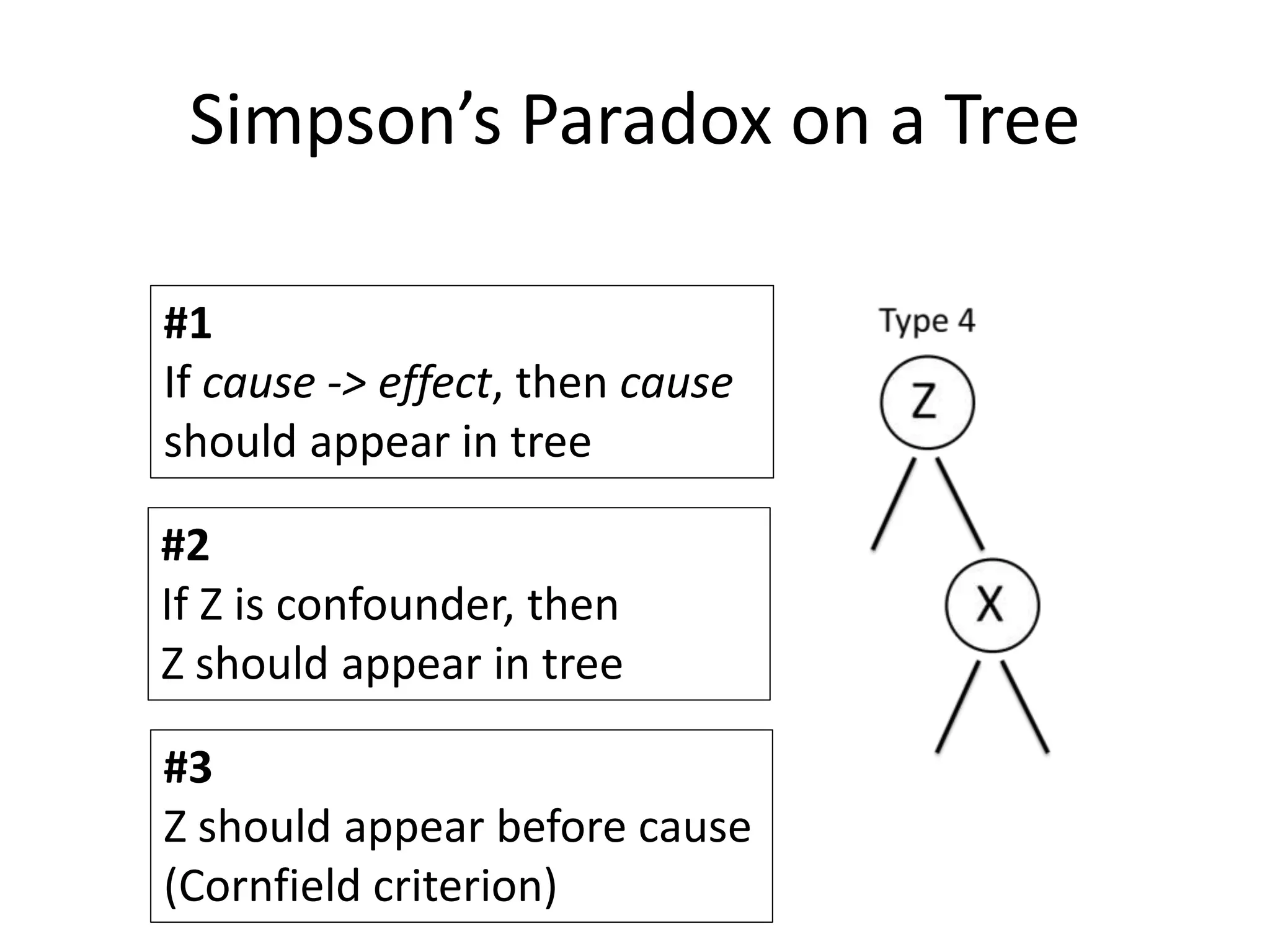
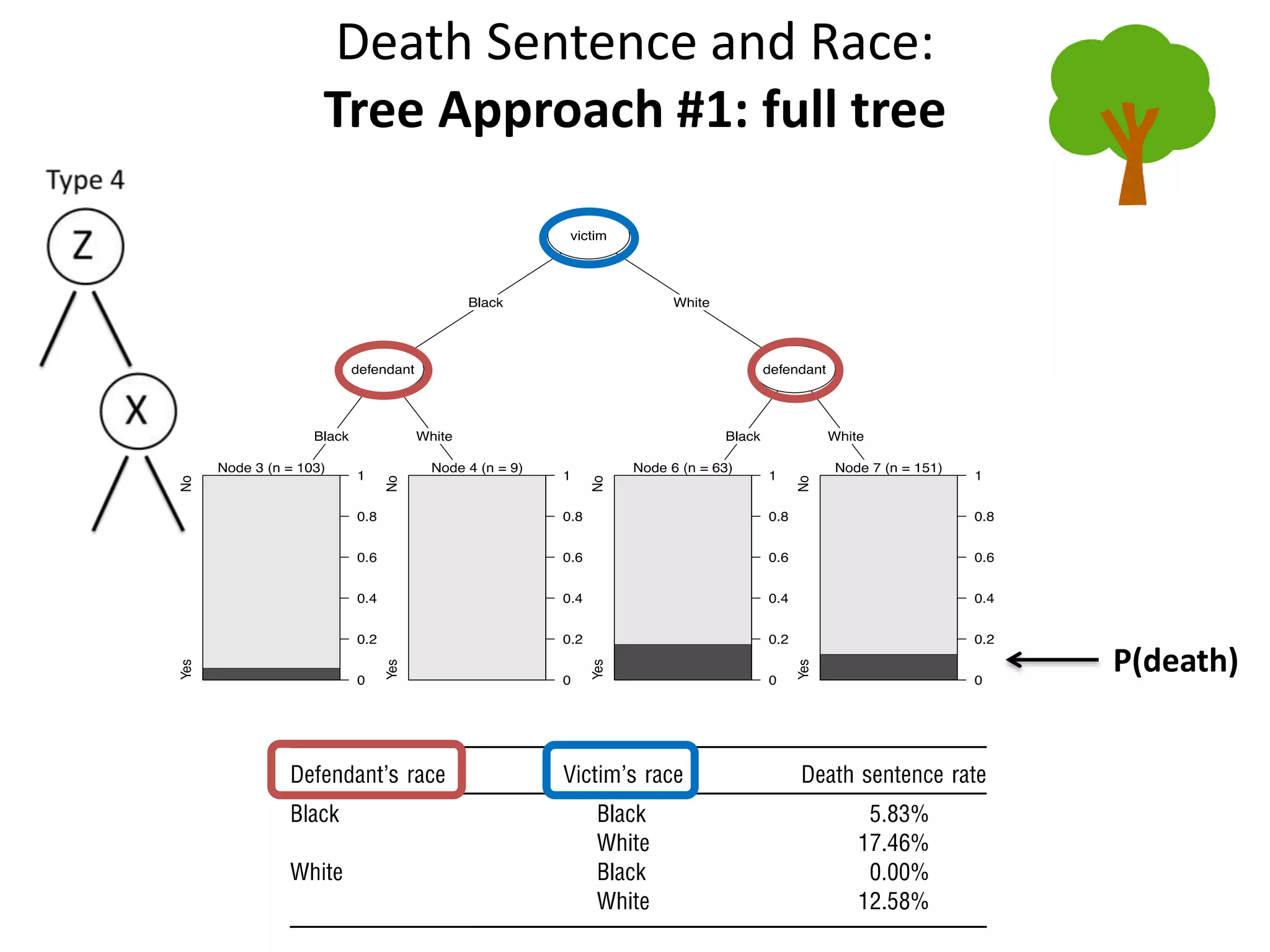
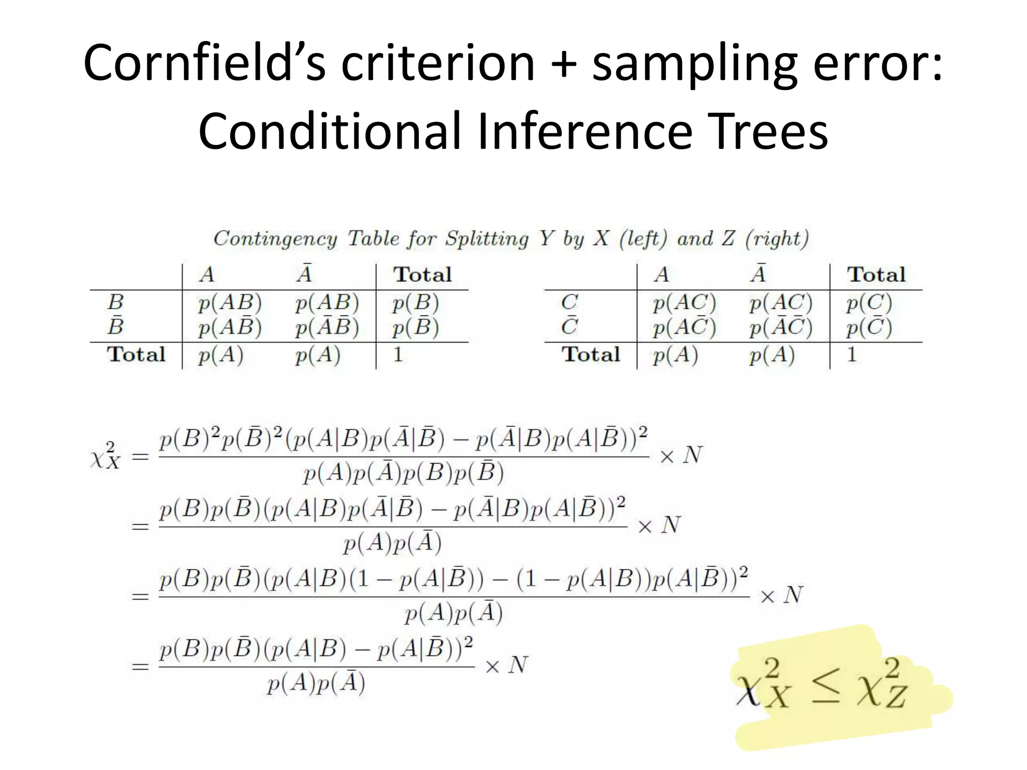
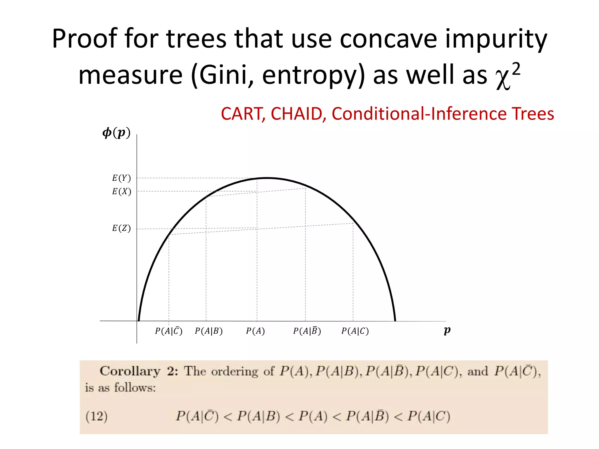
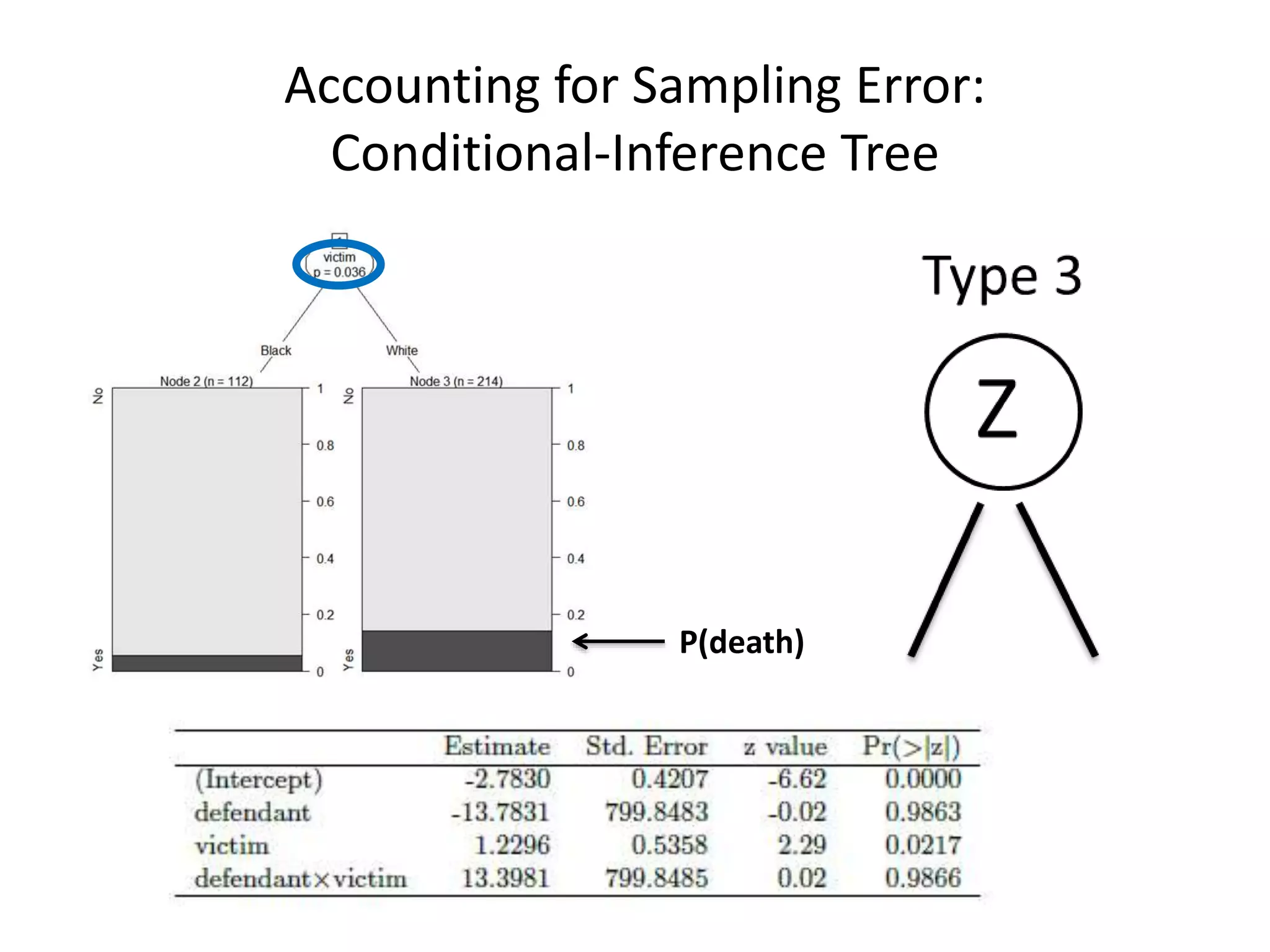
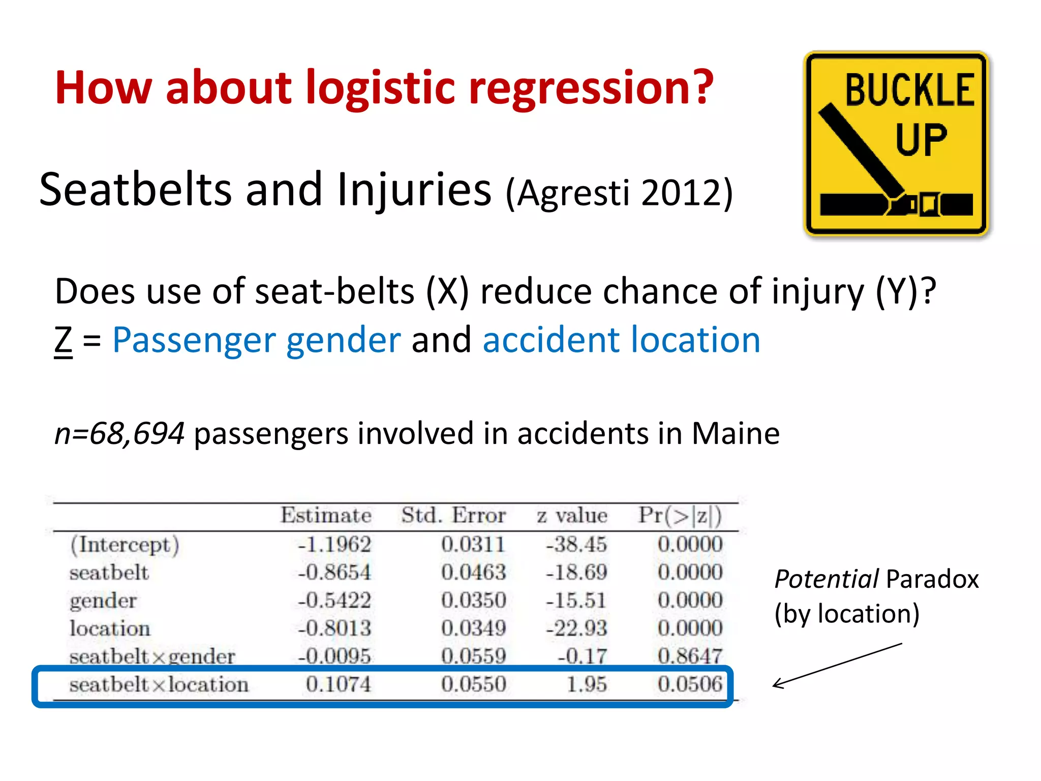
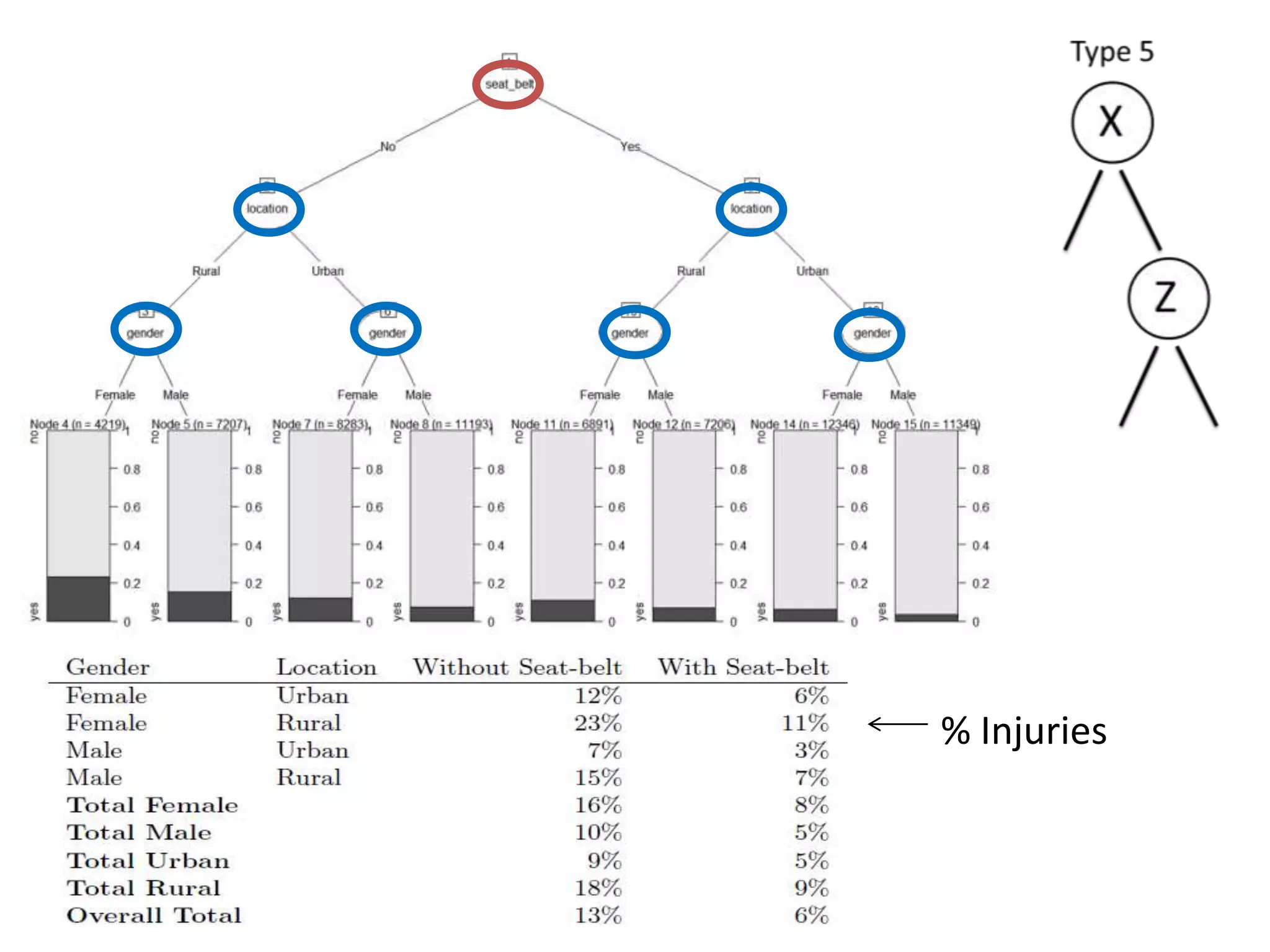
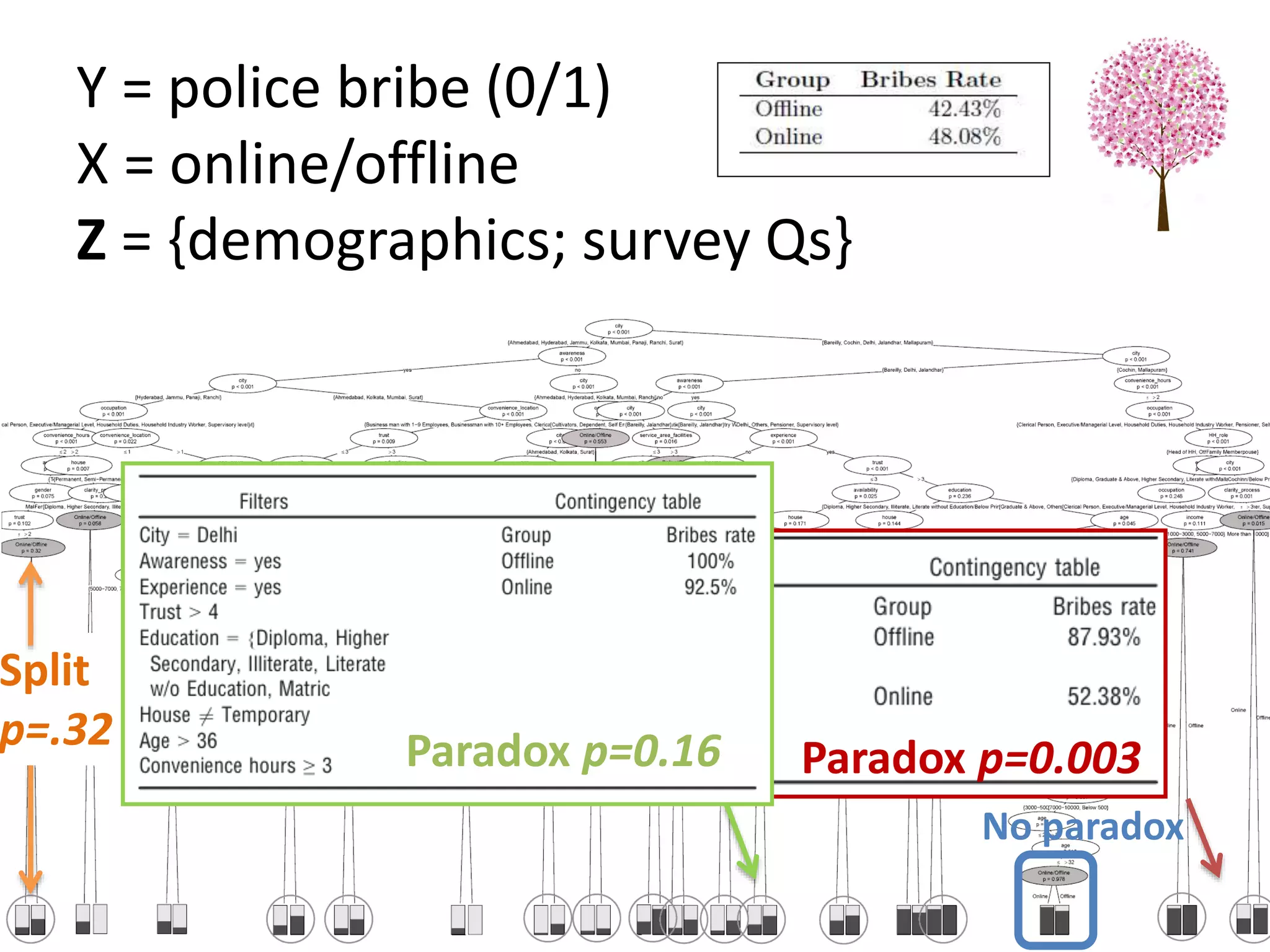
![Goal: Does a dataset exhibit SP?
C = confounder
E = effectA = cause
P (E|C ) – P( E|C’ ) P (E|A ) – P(E|A’ )
“If Cornfield’s minimum effect size is not reached,
[you] can assume no causality” Schield, 1999
Cornfield et al’s Criterion](https://image.slidesharecdn.com/treesforcausalresearchwombatmonashnov2019-191129032230/75/Repurposing-Classification-Regression-Trees-for-Causal-Research-with-High-Dimensional-Data-34-2048.jpg)

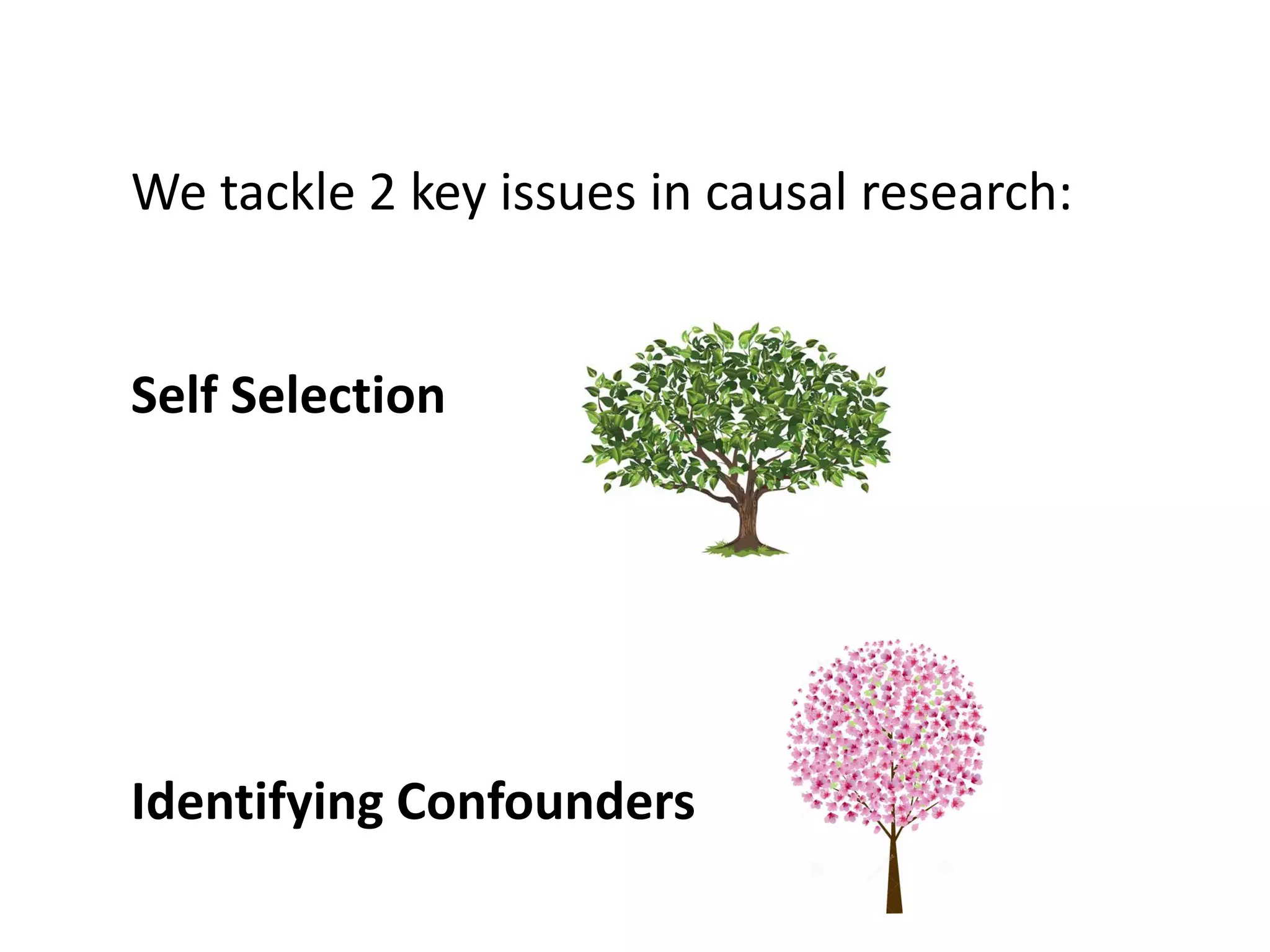


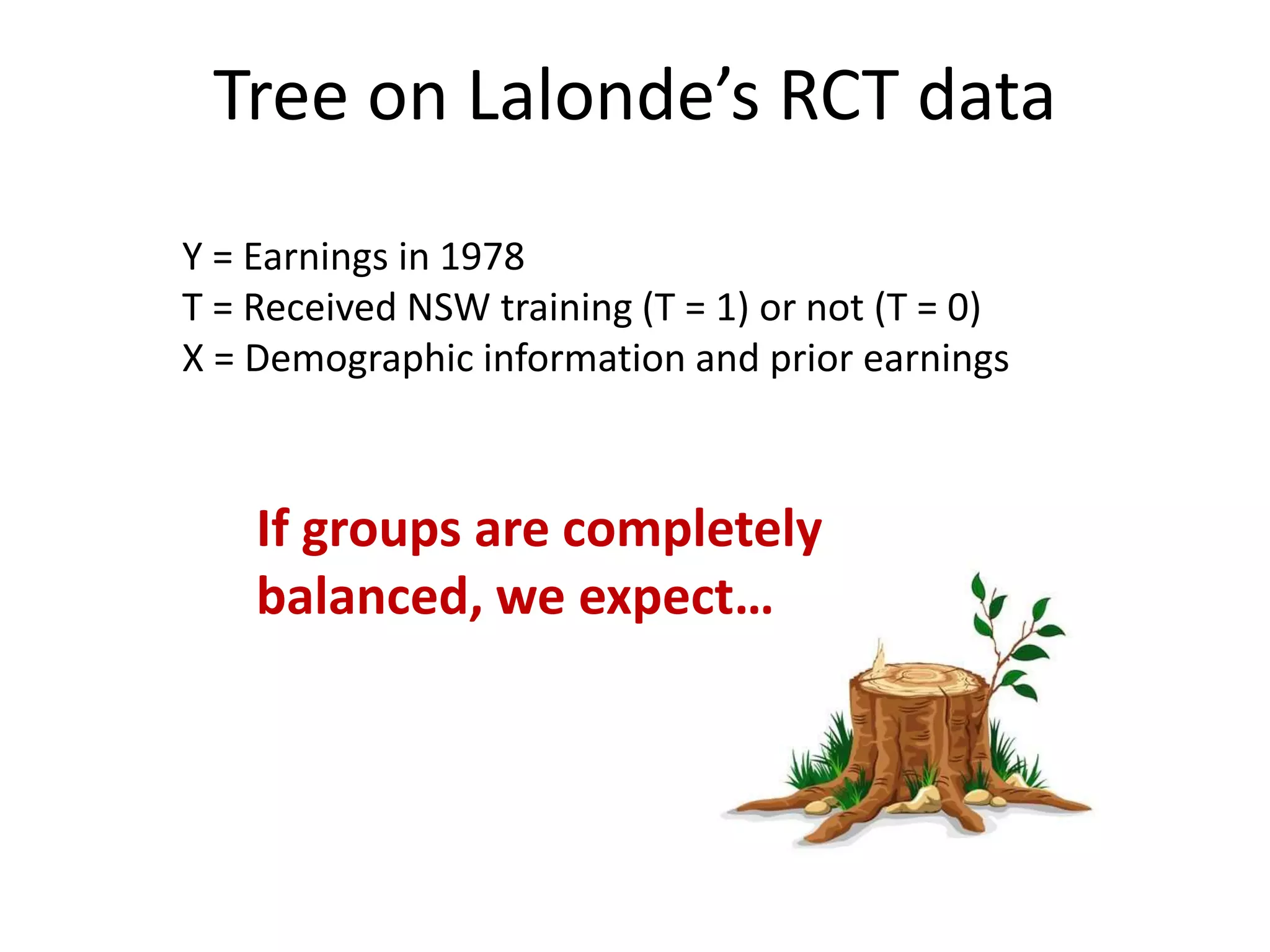
The document discusses a tree-based approach for addressing self-selection in causal research involving high-dimensional data, aimed at improving impact studies such as randomized experiments and quasi-experiments. It outlines the challenges of traditional propensity score methods in big data and proposes a new method that leverages classification and regression trees to identify confounders and analyze treatment effects more effectively. The authors present applications of this method in various domains, demonstrating its advantages over conventional techniques in detecting heterogeneous treatment effects and handling unbalanced covariates.


![[DSC Europe 25] Nikola Rajovic - Hardware Technologies Under the Hood: RISC-V...](https://cdn.slidesharecdn.com/ss_thumbnails/o2gptrmtoyqndgoshwgq-dsc2025-tenstorrent-rajovic-251205090438-814685f5-thumbnail.jpg?width=640&height=640&fit=bounds)

![[DSC Europe 25] Bogdan Daniel Maruneac - AI - It starts with you.pptx](https://cdn.slidesharecdn.com/ss_thumbnails/odov3snhrcqs9hx5ny2n-4-251205085715-f1daacfe-thumbnail.jpg?width=640&height=640&fit=bounds)
![[DSC Europe 25] Marija Vlajkovic & Andrea Radonjanin - Integration of AI tool...](https://cdn.slidesharecdn.com/ss_thumbnails/qf1jrglttoc3bm8s3aop-final-integration-of-ai-tools-251208151905-394f3a6a-thumbnail.jpg?width=640&height=640&fit=bounds)
![[DSC Europe 25] Dragana Ilic - AI for Big Data in Astronomy.pptx](https://cdn.slidesharecdn.com/ss_thumbnails/8palya86qaatvjhva1ms-2-dragana-ilic-ai-ilic-251208151906-652b819c-thumbnail.jpg?width=640&height=640&fit=bounds)


![[DSC Europe 25] Boris Perkovic - Lost in performance.pptx](https://cdn.slidesharecdn.com/ss_thumbnails/uq5hrp7vsuahqkxzifux-1-251204082258-fd2ee09d-thumbnail.jpg?width=640&height=640&fit=bounds)


![[DSC Europe 25] Max Talanov - Non digital NNs.pptx](https://cdn.slidesharecdn.com/ss_thumbnails/wif8tr3gtua74qvtopke-non-digital-nns-251205090438-26b0eea6-thumbnail.jpg?width=640&height=640&fit=bounds)


![[DSC Europe 25] Dusan Jovicic - AI Story: From on-prem to cloud and back agai...](https://cdn.slidesharecdn.com/ss_thumbnails/8kp49m6uq22ifnbwhfnk-2-251205085715-964d11a6-thumbnail.jpg?width=640&height=640&fit=bounds)
