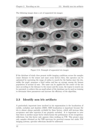
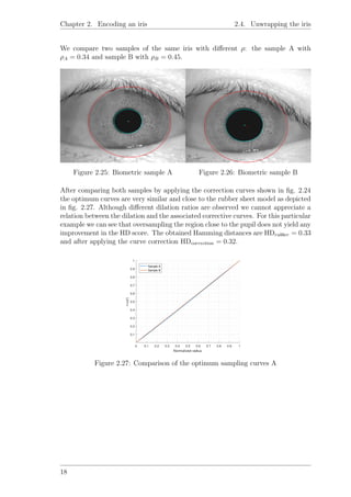
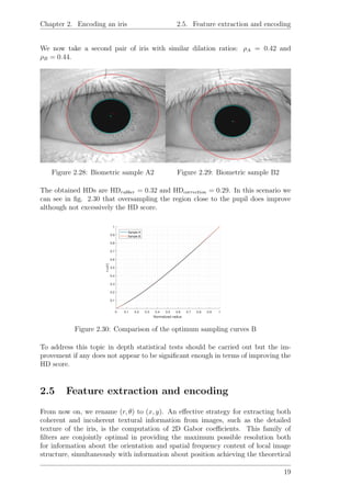
This document describes the implementation of an iris-based biometric system, including the theoretical basis and implementation methods studied from other documents. It discusses how iris recognition works by extracting characteristic patterns from iris images using mathematical techniques to generate iris codes for identification. The segmentation and normalization of iris images is challenging due to factors like eyelashes and pupil dilation. The prototype was created in Matlab but a real system would need a more efficient platform like C++.

1. UNIVERSITAT POLIT`ECNICA DE
CATALUNYA
Escola T`ecnica Superior d’Enginyeria de
Telecomunicaci´o de Barcelona
Grau en Enginyeria de Sistemes de Telecomunicaci´o
HUMAN IRIS BIOMETRY
Author:
Largo Castell`a,
Juan Carlos
Supervisor:
Dr. Villar Santos,
Jorge Luis
August 2, 2016

2. Abstract
This project exposes the implementation of an iris based biometric system, from the
theoretical basis to the implementation of it by examining different types of methods
described in other documents.
The human iris structure remains invariant over the time containing several easily
identifiable structures, believed to be unique to each person [1]. This information is
extracted by using mathematical pattern-recognition techniques to obtain a charac-
teristic iris code which can be used in identification systems.
The recognition principle is the failure of a test of statistical independence on the
iris codes since two different iris codes should not agree in more than a half of their
bits. The operating principle is as follows: first the system has to localize the inner
and outer boundaries of the iris (pupil and limbus) in an image of an eye. Further
subroutines detect and exclude eyelids, eyelashes, and specular reflections that often
occlude parts of the iris. The set of pixels containing only the iris, normalized
by a rubber-sheet model to compensate for pupil dilation or constriction, is then
analyzed to extract an iris code encoding the information needed to compare two iris
images. The code generated by imaging an iris is compared to stored template(s)
in a database. If the Hamming distance is below the decision threshold, a positive
identification outcomes due to the statistical improbability that two different persons
could agree by chance in so many bits, given the high entropy of iris templates.
The iris segmentation and normalization process is challenging due to the presence of
eyelashes, eyelids, and reflections that may occlude regions of the iris. Furthermore,
the dilation of pupils due to different light illuminations and the inconvenient that
the iris and the pupil are not concentric cause this type of biometry to be quite
complex.
I

3. Resumen
Este proyecto expone la implementaci´on de un sistema biom´etrico basado en el iris,
desde la base te´orica hasta la implementaci´on del mismo por mediante el estudio de
diferentes metodos descritos en otros documentos.
La estructura del iris humano permanece estable a lo largo del tiempo conteniendo
esta varias estructuras f´aciles de identificar, las cuales son consideradas ´unicas en
cada persona [1]. Dicha informaci´on es extraida mediante t´ecnicas matem´aticas de
reconocimiento de patrones para obtener as´ı un c´odigo asociado al iris que puede
ser utilizado en sistemas de autenticaci´on biom´etrica.
El principio de funcionamiento es el siguiente: primero el sistema tiene que localizar
los l´ımites interior y exterior del iris (la pupila y el limbo) en una imagen de un
ojo. Posteriores subrutinas detectan y excluyen los p´arpados, las pesta˜nas y las
reflexiones especulares que a menudo obstruyen partes del iris. El conjunto de
p´ıxeles que contienen ´unicamente el iris, normalizado por un modelo conocido como
“rubber sheet model” que compensa la dilataci´on o constricci´on de la pupila, es
analizado posteriormente para extraer un c´odigo del iris que codifica la informaci´on
necesaria para comparar dos im´agenes del iris. El c´odigo generado mediante las
im´agenes de un iris se compara con una o varias plantillas almacenadas en la base
de datos. Si la distancia de Hamming est´a por debajo del umbral de decisi´on, se
valida la identidad de cierto individuo debido a la improbabilidad estad´ıstica de que
dos personas diferentes puedan coincidir por casualidad en tantos bits del c´odigo,
dada la alta entrop´ıa de las plantillas del iris.
El proceso de segmentaci´on y normalizaci´on del iris supone un reto debido a la
presencia de pesta˜nas, p´arpados y reflexiones que pueden obstruir las regiones del
iris. Adem´as, la dilataci´on de la pupila debido a los diferentes niveles de iluminaci´on
y el inconveniente que el iris y la pupila no son conc´entricas conllevan que este tipo
de biometr´ıa sea bastante compleja.
II

4. Resum
Aquest projecte exposa la implementaci´o d’un sistema biom`etric basat en l’iris, des
de la base te`orica fins a la implementaci´o del mateix per mitj`a de l’estudi de diferents
m`etodes descrits en altres documents.
L’estructura de l’iris hum`a roman estable al llarg del temps contenint aquesta di-
verses estructures f`acils d’identificar, les quals s´on considerades ´uniques en cada
persona [1]. Tal informaci´o ´es extreta mitjan¸cant t`ecniques matem`atiques de re-
coneixement de patrons per obtenir aix´ı un codi associat a l’iris que pot ser emprat
en sistemes d’autenticaci´o biom`etrica.
El principi de funcionament ´es el seg¨uent: primer el sistema ha de localitzar els l´ımits
interior i exterior de l’iris (la pupil·la i el limb) en una imatge d’un ull. Posteriors
subrutines detecten i exclouen les parpelles, les pestanyes i les reflexions especulars
que sovint obstrueixen parts de l’iris. El conjunt de p´ıxels que contenen ´unicament
l’iris, normalitzat per un model conegut com ”rubber sheet model” que compensa la
dilataci´o o constricci´o de la pupil·la, ´es analitzat posteriorment per extreure un codi
de l’iris que codifica la informaci´o necess`aria per comparar dues imatges de l’iris.
El codi generat mitjan¸cant les imatges d’un iris es compara amb una o diverses
plantilles emmagatzemades en la base de dades. Si la dist`ancia de Hamming es
troba per sota del llindar de decisi´o, es valida la identitat de cert individu a causa
de la improbabilitat estad´ıstica que dues persones diferents puguin coincidir per
casualitat en tants bits del codi, donada l’alta entropia de les plantilles de l’iris.
El proc´es de segmentaci´o i normalitzaci´o de l’iris suposa un repte a causa de la
pres`encia de pestanyes, parpelles i reflexions que poden obstruir les regions de
l’iris. A m´es, la dilataci´o de la pupil·la a causa dels diferents nivells d’il·luminaci´o
i l’inconvenient que l’iris i la pupil·la no s´on conc`entriques comporten que aquest
tipus de biometria sigui bastant complexa.
III

5. State of the art
John Daugman settled down the basis of iris recognition systems back in 1994, when
he patented and published in a paper his algorithm for image processing, feature
extraction, and matching.
The principle of iris recognition is based on a failure of a test of statistical inde-
pendence on iris phase structure projected under 2D Gabor wavelet filters. The
combinatorial complexity of this phase information across different persons presents
high enough entropy among samples from different classes (different iris) to provide
reliable decisions about personal identity with extremely high confidence.
IV

6. Statement of the purpose
The purpose of this project is to understand the fundamentals of iris recognition
systems. How are these methods implemented, what does the recognition rely on,
how are these methods used and what do these methods achieve along with their
limitations.
An implementation of an iris recognition system is carried on along this project,
trying to replicate in the best possible way the results achieved by John Daugman.
The prototype code has been written under Matlab R2016a but for a real application
scenario C++ or other more efficient platforms should be considered.

7. Contents
1 Introduction to biometrics 1
1.1 Anatomy of the human eye . . . . . . . . . . . . . . . . . . . . . . . . 2
1.1.1 The iris . . . . . . . . . . . . . . . . . . . . . . . . . . . . . . 3
1.1.2 The pupil . . . . . . . . . . . . . . . . . . . . . . . . . . . . . 4
1.2 Iris biometry . . . . . . . . . . . . . . . . . . . . . . . . . . . . . . . 5
2 Encoding an iris 6
2.1 Locating the pupil . . . . . . . . . . . . . . . . . . . . . . . . . . . . 7
2.1.1 Binarization . . . . . . . . . . . . . . . . . . . . . . . . . . . . 7
2.1.2 The Canny edge detector . . . . . . . . . . . . . . . . . . . . . 8
2.1.3 Circular Hough transform . . . . . . . . . . . . . . . . . . . . 9
2.2 Locating the limbus . . . . . . . . . . . . . . . . . . . . . . . . . . . . 10
2.3 Identify non iris artifacts . . . . . . . . . . . . . . . . . . . . . . . . . 12
2.4 Unwrapping the iris . . . . . . . . . . . . . . . . . . . . . . . . . . . . 13
2.4.1 Rubber sheet model . . . . . . . . . . . . . . . . . . . . . . . 14
2.4.2 Bio-mechanical model . . . . . . . . . . . . . . . . . . . . . . 15
2.4.3 Discussion . . . . . . . . . . . . . . . . . . . . . . . . . . . . . 17
2.5 Feature extraction and encoding . . . . . . . . . . . . . . . . . . . . . 19
3 Matching iris codes 22
3.1 Achieving orientation invariance . . . . . . . . . . . . . . . . . . . . . 24
3.2 Performance of the code . . . . . . . . . . . . . . . . . . . . . . . . . 25
4 Experimental results 26
4.1 Database characterization . . . . . . . . . . . . . . . . . . . . . . . . 27
4.2 Code sensitivity . . . . . . . . . . . . . . . . . . . . . . . . . . . . . . 29
4.3 Statistic results . . . . . . . . . . . . . . . . . . . . . . . . . . . . . . 32
5 Conclusions and future work 34

8. List of Figures
1.1 Steps in a biometric system (1) . . . . . . . . . . . . . . . . . . . . . 1
1.2 Steps in a biometric system (2) . . . . . . . . . . . . . . . . . . . . . 1
1.3 Eye anatomy . . . . . . . . . . . . . . . . . . . . . . . . . . . . . . . 2
1.4 Iris muscles . . . . . . . . . . . . . . . . . . . . . . . . . . . . . . . . 3
1.5 Iris texture . . . . . . . . . . . . . . . . . . . . . . . . . . . . . . . . 4
2.1 ROI extraction process. . . . . . . . . . . . . . . . . . . . . . . . . . . 6
2.2 Encoding process. . . . . . . . . . . . . . . . . . . . . . . . . . . . . . 6
2.3 Pupil location process . . . . . . . . . . . . . . . . . . . . . . . . . . 7
2.4 Original biometric sample . . . . . . . . . . . . . . . . . . . . . . . . 7
2.5 Binarized biometric sample . . . . . . . . . . . . . . . . . . . . . . . . 7
2.6 Canny input sample . . . . . . . . . . . . . . . . . . . . . . . . . . . 8
2.7 Canny edge response . . . . . . . . . . . . . . . . . . . . . . . . . . . 8
2.8 2D circular Hough transform . . . . . . . . . . . . . . . . . . . . . . . 10
2.9 3D circular Hough transform . . . . . . . . . . . . . . . . . . . . . . . 10
2.10 Biometric sample with soft iris transition towards sclera . . . . . . . . 11
2.11 Biometric sample with double limbic boundary . . . . . . . . . . . . . 11
2.12 Segmented iris from image 2.10 . . . . . . . . . . . . . . . . . . . . . 11
2.13 Segmented iris from image 2.11 . . . . . . . . . . . . . . . . . . . . . 11
2.14 Example of segmented iris images . . . . . . . . . . . . . . . . . . . . 12
2.15 Points to fit in parabola . . . . . . . . . . . . . . . . . . . . . . . . . 13
2.16 Eyelid segmentation . . . . . . . . . . . . . . . . . . . . . . . . . . . 13
2.17 Example of the normalization of an iris . . . . . . . . . . . . . . . . . 14
2.18 Rubber sheet model meshwork . . . . . . . . . . . . . . . . . . . . . . 15
2.19 Rubber sheet model crosslinks . . . . . . . . . . . . . . . . . . . . . . 15
2.20 Bio-mechanical model radial displacement prediction for ρ = 0.75 . . 16
2.21 Bio-mechanical model final position prediction for ρ = 0.75 . . . . . . 16
2.22 Bio-mechanical model meshwork for ρ = 0.75 . . . . . . . . . . . . . . 16
2.23 Rubber sheet model meshwork for ρ = 0.75 . . . . . . . . . . . . . . . 16
2.24 Set of correction curves . . . . . . . . . . . . . . . . . . . . . . . . . . 17
2.25 Biometric sample A . . . . . . . . . . . . . . . . . . . . . . . . . . . . 18
2.26 Biometric sample B . . . . . . . . . . . . . . . . . . . . . . . . . . . . 18
2.27 Comparison of the optimum sampling curves A . . . . . . . . . . . . 18
2.28 Biometric sample A2 . . . . . . . . . . . . . . . . . . . . . . . . . . . 19
2.29 Biometric sample B2 . . . . . . . . . . . . . . . . . . . . . . . . . . . 19
2.30 Comparison of the optimum sampling curves B . . . . . . . . . . . . 19
2.31 Gabor filter bank . . . . . . . . . . . . . . . . . . . . . . . . . . . . . 20

9. List of Figures List of Figures
3.1 HD distribution of uncorrelated iris . . . . . . . . . . . . . . . . . . . 23
3.2 Observed vs Binomial cumulatives . . . . . . . . . . . . . . . . . . . . 23
3.3 Original HD distribution . . . . . . . . . . . . . . . . . . . . . . . . . 25
3.4 Rotated HD distribution . . . . . . . . . . . . . . . . . . . . . . . . . 25
4.1 Distribution of shifts for x axis . . . . . . . . . . . . . . . . . . . . . 27
4.2 Distribution of shifts for y axis . . . . . . . . . . . . . . . . . . . . . . 27
4.3 Distance from limbic center relative to pupil radius . . . . . . . . . . 27
4.4 Distribution of pupil radius . . . . . . . . . . . . . . . . . . . . . . . 28
4.5 Distribution of limbus radius . . . . . . . . . . . . . . . . . . . . . . . 28
4.6 Distribution of dilation ratios (ρ) . . . . . . . . . . . . . . . . . . . . 28
4.7 Code shift distribution of uncorrelated iris . . . . . . . . . . . . . . . 29
4.8 Code shift distribution of same iris . . . . . . . . . . . . . . . . . . . 29
4.9 Decision environment at θ = 0 without angular correction . . . . . . . 29
4.10 Decision environment at θ = 0 after angular correction . . . . . . . . 29
4.11 Decision environment at θ = 90 without angular correction . . . . . . 30
4.12 Decision environment at θ = 90 after angular correction . . . . . . . . 30
4.13 Code sensitivity at θ = 0 . . . . . . . . . . . . . . . . . . . . . . . . . 30
4.14 Code sensitivity at θ = 90 . . . . . . . . . . . . . . . . . . . . . . . . 30
4.15 Decidability . . . . . . . . . . . . . . . . . . . . . . . . . . . . . . . . 32
4.16 True positives (TP) . . . . . . . . . . . . . . . . . . . . . . . . . . . . 33
4.17 Decision environment at λ = 10 . . . . . . . . . . . . . . . . . . . . . 33
4.18 Decision environment at λ = 15 . . . . . . . . . . . . . . . . . . . . . 33

10. Chapter 1
Introduction to biometrics
Biometrics refers to metrics related to human characteristics which can be used to
measure and describe physiological and behavioural characteristics of an individual.
Some examples of physiological characteristics include, but are not limited to finger-
print, face, palm print, iris, retina, among others. As previously mentioned, it may
seem that most biometric systems are image-based, but not all, voice for example
requires spectral analysis to perform biometric identification. These traits can be
used to identify an individual and provide reliable automatic recognition of persons.
The principal steps in a biometric system can be described by the following chart:
Biometric
sample
ROI
segmentation
Feature
extraction
Characteristic
vector
Figure 1.1: Steps in a biometric system (1)
Once the characteristic vector is extracted from the biometric sample, it is commonly
encrypted to prevent possible data filtration which can lead to impersonation of
identity. Finally, the characteristic vector is then compared with a database of
characteristic vectors to validate the identity of an individual, such vector may
have or not been encrypted previously. In case the system relies on encryption the
matching procedure must act accordingly by decrypting at the time of matching or
by working with homomorphic encryption.
Characteristic
vector
Matching Decision
Database
Figure 1.2: Steps in a biometric system (2)
1

11. Chapter 1. Introduction to biometrics 1.1. Anatomy of the human eye
The matching criteria relies on a characteristic and unique pattern associated to
the individual. The key issue associated to all pattern recognition problems is the
relation between inter-class and intra-class variability: objects can be reliably clas-
sified only if the variability among different instances of a given class is significantly
less than the variability between different classes. For example, in face recognition,
difficulties arise from the fact that the face is a changeable social organ displaying
a variety of expressions, as well as being an active three-dimensional object whose
image varies with viewing angle, pose, age and other factors. Against this intra-
class (same face) variability, inter-class variability is limited because different faces
possess the same basic set of features, in the same canonical geometry such as the
case of monozygotic twins. Similar problems arise when dealing with fingerprint
biometrics, since the fingerprints are often subject to handwork and labour and can
become harmed introducing marks or modifying the original fingerprint. The iris
instead, presents a much wider range of characteristics that present an enormous
variability (since some characteristics may or may not be present in an iris), is well
protected from the environment since it is an internal (yet externally visible) organ
of the eye and is stable over time reaching its final shape on the eighth month of
gestation of a human being. For all of these reasons, iris patterns become interesting
as an alternative approach to reliable recognition of persons.
1.1 Anatomy of the human eye
The external eye is composed by two main pieces. The smaller frontal part, trans-
parent and more curved, called the cornea, is linked to the larger white unit called
the sclera. The sclerotic chamber constitutes the remaining region of the eye. It
has a white color and its radius is typically about 12 mm. The cornea and sclera
are connected by a ring called the limbus. The iris is the colored circular structure
concentrically surrounding the center of the eye and finally, the pupil, which appears
to be black. The size of the pupil controls the amount of light entering the eye.
Figure 1.3: Eye anatomy
The eyeball grows rapidly, increasing from about 16–17 millimetres at birth to
22.5–23 mm by three years of age. By age 13, the eye attains its full size of around
24 mm, dimensions differ among adults by only one or two millimetres, staying
remarkably consistent across different ethnicities.
2

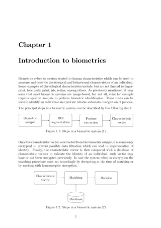
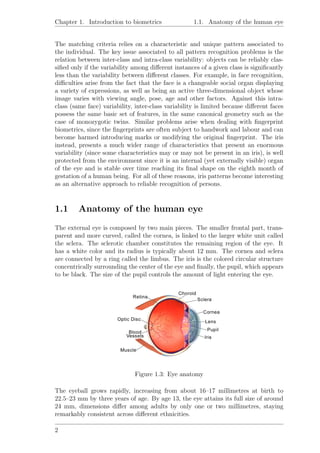
12. Chapter 1. Introduction to biometrics 1.1. Anatomy of the human eye
1.1.1 The iris
There are some important aspects of the iris which are to be considered when build-
ing a biometric system: which is its anatomic structure?, is this structure genetically
bound?, when does it attain its maturity?, does its texture remain invariant over
time?. Some of these aspects may help understand the limitations associated to iris
biometric systems.
The iris has a fixed diameter with an average of 12 mm among the population, it
is a muscular tissue responsible for controlling the diameter and size of the pupil
and thus the amount of light reaching the retina. There are two groups of smooth
muscles for this purpose: a circular group called the sphincter pupillae, and a radial
group called the dilator pupillae. This can be seen in fig. 1.4.
Figure 1.4: Iris muscles
The iris begins to form in the third month of gestation and the structures creating
its pattern are largely complete by the eighth month, although pigment accretion
can continue into the first postnatal years. Its complex pattern can contain many
distinctive features such as arching ligaments, furrows, ridges, crypts, rings, corona,
freckles, and a zigzag collarette, some of which can be seen in fig. 1.4. Statistical
tests of iris texture demonstrate that the patterns associated to each individual are
not genetically bound[1] whilst the color of the iris is strongly determined genetically,
this means that even monozygotic twins which posses identical DNA will present
different iris texture. Furthermore, the two eyes of an individual contain completely
independent iris patterns.
3

13. Chapter 1. Introduction to biometrics 1.1. Anatomy of the human eye
Figure 1.5: Iris texture
The surface of the multilayered iris that is visible includes two sectors that are
different in color, an outer ciliary part and an inner pupillary part. These two parts
are divided by the collarette which appears as a zigzag pattern.
The striated tabecular meshwork of elastic pectinate ligament creates the predom-
inant texture under visible light, whereas in the near-infrared (NIR) wavelengths
slowly modulated stromal features dominate the iris pattern. In NIR wavelengths,
even darkly pigmented irises reveal rich and complex features.
1.1.2 The pupil
The pupil is the opening in the centre of the eye which allows light to strike the
retina. Light enters through the pupil and goes through the lens, which focuses
the image on the retina. The reason why the pupil appears black is due to light
rays entering the pupil are either absorbed by the tissues inside the eye directly, or
absorbed after diffuse reflections within the eye that mostly miss exiting the narrow
pupil. In optical terms, the anatomical pupil is the eye’s aperture and the iris is
the aperture stop adapting in diameter to allow more or less light to reach the
retina. When more light is needed, the pupil gets dilated (process known as miosis)
and when there is an excess of light reaching the retina the pupil gets constricted
(process known as mydriasis). The normal pupil size in adults varies from 2 to 4 mm
in diameter when constricted to 4 to 8 mm when dilated, taking in consideration
that the diameter of the iris is fixed around 12 mm, the expected dilation ratio
defined as:
ρ =
pupil diameter
iris diameter
(1.1)
Parameter ρ is thereby expected to be comprised between ρ ∈ [0.15, 0.7]. The pupil
and the limbus are not concentric, in fact, the pupil center tends to be shifted
towards the nasal region and it is not unusual to observe shifts of around 20% of the
4

14. Chapter 1. Introduction to biometrics 1.2. Iris biometry
pupil radius. Research shows that the pupil center is related to its constriction[2],
becoming the limbus and pupil more concentric the more the pupil gets dilated.
Besides from the changes in size experienced by the pupil determined by ambient
illumination, focal length, drug action, emotional conditions, among others, the
pupil is also subject to rhythmic, but regular variations in diameter, called hippus,
occurring in a frequency range of 0.05 to 0.3Hz. This phenomena is independent of
eye movements or changes in illumination and is particularly noticeable when pupil
function is tested with a light.
1.2 Iris biometry
First of all, the biometric system has to localize the inner and outer boundaries of
the iris (pupil and limbus) on the image of an eye. Further subroutines detect and
exclude eyelids, eyelashes, and specular reflections that often occlude parts of the
iris. The set of pixels containing only the iris, normalized by a rubber-sheet model
to compensate for pupil dilation or constriction, is then analyzed to extract a bit
pattern encoding the information needed to compare two iris images.
For identification (one-to-many template matching) or verification (one-to-one tem-
plate matching), the resultant code obtained by imaging an iris is compared to stored
template(s) in a database. If the Hamming distance is below the decision threshold,
a positive identification has effectively been made because of the statistical extreme
improbability that two different persons could agree by chance in so many bits, given
the high entropy of iris templates.
A minimum of information is expected to capture the rich details of iris patterns,
therfore an imaging system should resolve a minimum of 70 pixels in iris radius[1].
An individual with darkly pigmented irises exhibits a low contrast between the pupil
and the iris region if the image is acquired under natural light, making segmentation
more difficult, for this reason NIR imaging is desirable, furthermore the majority of
persons worldwide have “dark brown eyes”, the dominant phenotype of the human
population, revealing less visible texture in the visible wavelength (VW) band but
appearing richly structured in the NIR band. Using the NIR spectrum also enables
the blocking of corneal specular reflections from a bright ambient environment, by
allowing only those NIR wavelengths from the narrow-band illuminator back into
the iris camera. An inconvenient when working with NIR imaging is that the limbic
boundary usually has extremely soft contrast when long wavelength NIR illumina-
tion is used, causing the segmentation of the iris to become more complicated.
5

15. Chapter 2
Encoding an iris
An iris biometric system firstly has to resolve the location of the region of interest
(ROI), by locating the inner and outer boundaries of the iris (pupil and limbus) in
an image of an eye. The ROI extraction relies on a proper identification of the pupil.
The reason for this is that it is the most distinctive and easy part to identify in the
eye and also bounds the region in which the limbus should be present. A proper
biometric sample has to provide enough information to identify the pupil correctly,
otherwise the image sample is discarded. Further subroutines detect and exclude
eyelids, eyelashes, and shadows that often occlude parts of the iris.
Locate the
pupil
Locate
the iris
Identify non
iris artifacts
Figure 2.1: ROI extraction process.
Once the ROI has been located, the set of pixels containing only the iris are then
normalized to compensate for pupil dilation or constriction and non concentricity
of the iris and the pupil in a process known as iris unwrapping. The normalized
iris is then projected under 2D Gabor wavelets to extract the texture information of
the iris. The projected iris is finally binarized to extract an iris code encoding the
information needed to compare two iris images.
ROI
segmentation
Unwrap
the iris
Feature
extraction
Iris
code
Figure 2.2: Encoding process.
In this thesis two iris unwrapping models have been studied to attempt to compen-
sate for pupil dilation and constriction. The first model called rubber sheet model
proposed by J. Daugman that compensates for pupil dilation without considering
the dilation ratio, and a second model called bio-mechanical model that considers
the dilation and adjusts the interpolation grid accordingly to the dilation.
6

16. Chapter 2. Encoding an iris 2.1. Locating the pupil
2.1 Locating the pupil
When looking for the pupil there are two main characteristics which can be exploited
to locate it: the pupil is one of the darkest regions in the eye and it is circular
shaped. Therefore, the main steps to carry on are segmenting the sample to identify
the dark regions (binarization) and then look for circles. The search for circular
shaped regions is efficiently achieved by the circular Hough transform (CHT) but
rather than looking for circles in the binarized image, its input is an edge response
image provided by the Canny edge detector to reduce the amount of information.
The overall process can be described by the following chart:
Figure 2.3: Pupil location process
Biometric
sample
Binarization
Canny edge
detector
Circular
Hough Tr.
2.1.1 Binarization
The binarization process takes an image, say I, and applies a certain threshold Ith.
Such threshold is adjusted through experimental analysis to extract only the dark
regions of the biometric sample. The binarization function is defined as:
IB(x, y) =
1 if I(x, y) < Ith
0 otherwise
(2.1)
In fig. 2.4 we can see the original iris sample and in fig. 2.5 the result of the
binarization with Ith.
Figure 2.4: Original biometric sample Figure 2.5: Binarized biometric sample
7

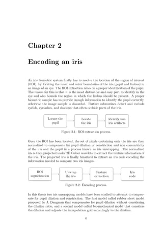
17. Chapter 2. Encoding an iris 2.1. Locating the pupil
2.1.2 The Canny edge detector
The purpose of edge detection is to significantly reduce the amount of data in an
image, while preserving the structural properties to be used for further image pro-
cessing. Canny’s edge detector uses a multi-stage algorithm to detect a wide range
of edges in images. The Process of Canny edge detection algorithm can be broken
down to 5 different steps:
1. Noise suppression: smooth the image using a Gaussian filter to reduce noise.
2. Finding gradients: apply Sobel operator to find image gradients.
3. Non-maximum suppression: preserve all local maximum edge values in the
gradient image and suppress the rest.
4. Double threshold: edge pixels stronger than the high threshold are marked
as strong; edge pixels weaker than the low threshold are suppressed and edge
pixels between the two thresholds are marked as weak.
5. Hysteresis: strong edges are interpreted as “true edges” and weak edges are
included if and only if they are connected to strong edges.
The resultant image after applying Canny edge detection to the image seen on 2.6
is shown on fig. 2.7. A detailed description of the Canny edge detector steps can be
found on references [3] and the original John F. Canny description from Canny at
[4].
Figure 2.6: Canny input sample Figure 2.7: Canny edge response
8

18. Chapter 2. Encoding an iris 2.1. Locating the pupil
2.1.3 Circular Hough transform
Hough transform (HT) algorithms can be used to determine the parameters of simple
parameterizable structures, such as lines, circles, ellipses and parabolas present in
an image. The Circular Hough transform (CHT) is designed to find a circle by
characterizing its center (x0, y0) and radius r0 in the parameter space. The equation
that defines a circle is given by:
(x − x0)2
+ (y − y0)2
= r2
0 (2.2)
Where x and y are the points of the circle on the image. The parametric form of
this circle equation is given by the following expressions:
x = x0 + r0 × cos(θ) (2.3)
y = y0 + r0 × sin(θ) (2.4)
In CHT method, for each edge point (xi, yi) a circle, say C, with radius rc is drawn
considering (xi, yi) as the center. Consider an arbitrary point p = (xc, yc) on C, then
the circle centered on (xc, yc) with radius rc must be passed through (xi, yi). To find
the desired circle, majority voting technique (i.e., Hough Transform) is applied. In
this process, for each point on C the accumulator value is increased by one. For
each edge points (xi, yi) : i = 1, 2, 3..., n, the HT is defined as:
H(xc, yc, rc) = h(xi, yi, xc, yc, rc) (2.5)
Where:
h(xi, yi, xc, yc, rc) =
1 if g(xi, yi, xc, yc, rc) = 0
0 otherwise
(2.6)
With:
C: g(xi, yi, xc, yc, rc) = (xi − xc)2
+ (yi − yc)2
− r2
c (2.7)
9

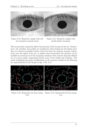
19. Chapter 2. Encoding an iris 2.2. Locating the limbus
The parameter triple (xc, yc, rc) that maximizes is common to the largest number
of edge points and is a reasonable choice to represent the circular contour. In figs.
2.8, 2.9 the CHT of the image obtained in 2.7 can be seen.
Figure 2.8: 2D circular Hough transform Figure 2.9: 3D circular Hough transform
The peak value corresponds to the center candidate of the voting procedure for a
given radius.
2.2 Locating the limbus
The parameters of the pupil can now be used to estimate the iris parameters since the
pupil and iris center present an offset which bounds the area in which a healthy iris
shall be contained. The radius of the iris is also bounded by the extreme dilation
ratios (ρ) of the pupil. Therefore, the procedure for locating the iris starts from
the parameters of the pupil. Then, it searches for the circular path where there
is maximum change in pixel values of the circular contour over the blurred partial
derivative of the edge image obtained from the Canny edge detector by varying
the radius between rpup × [1.2, 1.8] and shifting the center in the region contained
in (xp, yp) ± 0.2 × rpup . The blurring over the edge response provides a higher
tolerance for deviations to take place over the contour image caused by digitization
of the pixels and to reduce the negative effect of the eccentricity of the iris. The
operator can be described by the following equation:
max
(r,x0,y0)
Gσ(r) ∗
∂
∂r r,x0,y0
I(x, y)
2πr
ds (2.8)
Where ∗ denotes the convolution product and d is the distance with respect to the
pupil center in pixels. This operator behaves as a circular edge detector to identify
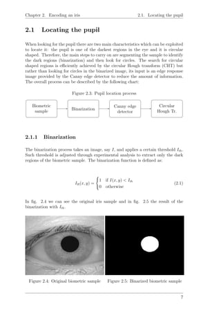
the outer limit of the iris (limbus). Locating the iris can become very difficult
since some iris present a soft transition towards the sclera when imaging in the NIR
spectrum, this can be seen in fig. 2.10 and other iris present an outer and inner
limbic boundary such as in fig. 2.11.
10

20. Chapter 2. Encoding an iris 2.2. Locating the limbus
Figure 2.10: Biometric sample with soft
iris transition towards sclera
Figure 2.11: Biometric sample with
double limbic boundary
This inconvenient negatively affects the precision of the location of the iris. Further-
more, the eyelashes and eyelids are troublesome when looking for the limbus since
they are treated as possible borders of the iris when the operator searches exhaus-
tively over the region of the eye, to address that inconvenient the operator can be
modified to search just over the maximum variation of the contour along the defined
arc of a given radius, suppressing thereby most of the eyelids and eyelashes. The
result of applying the proper modifications to the operator resulted in the following
iris segmentations for the images in figs. 2.10, 2.11:
Figure 2.12: Segmented iris from image
2.10
Figure 2.13: Segmented iris from image
2.11
11

21. Chapter 2. Encoding an iris 2.3. Identify non iris artifacts
The following images show a set of segmented iris images:
Figure 2.14: Example of segmented iris images
If the database of study does present stable imaging conditions across the samples
(same distance to the sensor and same zoom factor) then, this operator can be
optimized by narrowing the range of radius to search for the limbus since the iris,
unlike the pupil, possesses a fixed radius and has an average among the human
population of around 12 mm. The same can be applied for the center of the iris
since according to the distance to the sensor and the zoom, the region to search can
be narrowed, to achieve this an small subset of the database can be used as training
to determine these parameters and increase the efficiency of the algorithm.
2.3 Identify non iris artifacts
A particularly important issue involved in iris segmentation is the localization of
eyelids, eyelashes and shadows (EES). EES localization is important because the
iris is almost always partially occluded by these factors, which will increase false
acceptance and false rejection if not properly excluded. It is important to note
that there is another major factor which harms the performance of iris recognition:
reflections; but this factor only appears when working on VW. This project aims
only samples obtained on the NIR spectrum for practical reasons but under VW
imaging systems, specular reflections should be addressed.
12

22. Chapter 2. Encoding an iris 2.4. Unwrapping the iris
Efficient EES localization is difficult. First, accurate eyelid localization is challenging
due to eyelashes occlusion and second; the variation of the intensity, amount and
shape irregularity of eyelashes. There are two ways to address EES localization:
establishing an eyelid curvature model statistically and a common arc structure to
identify eyelashes or excluding a predefined region of the iris. Although one method
is more desirable than the other we have to consider that EES localization accuracy
is not faultless and it has time consumption associated to image processing whilst
excluding a predefined region of the iris has no computational cost but the expense
of discarding relevant information.
In this project a first approach to eyelid localization was tackled by performing a
rectangular average filter followed by Sobel horizontal filter which is then binarized
by using a threshold determined by experimental analysis. The points within pupil
and outside of the iris are suppressed, the resultant points are then used to fit a
parabola.
Figure 2.15: Points to fit in parabola Figure 2.16: Eyelid segmentation
The implemented method was proposed by Basit et al. on [5]. The reason for
implementing this method was because of its simplicity but it did not provide the
desired results. For this reason other more accurate and complex methods should be
explored, some of which can be seen seen on [6, 7, 8, 9]. Instead of addressing EES, a
predefined region of the iris was discarded from comparison but further development
of this project should properly address EES.
2.4 Unwrapping the iris
Robust representations for pattern recognition must be invariant to changes in the
size, position, and orientation of the patterns. In the case of iris recognition, this
means we must create a representation that is invariant to the optical size of the
iris in the image (which depends upon the distance to the eye, and zoom), the size
of the pupil within the iris (which introduces a non affine pattern deformation), the
location of the iris within the image, and the iris orientation, which depends upon
head tilt, torsional eye rotation within its socket, and camera angles. Fortunately,
invariance to all of these factors can readily be achieved.
13

23. Chapter 2. Encoding an iris 2.4. Unwrapping the iris
For on-axis but possibly rotated iris images, it is natural to use a projected pseudo-
polar coordinate system. The polar coordinate grid is not necessarily concentric,
since in most eyes the pupil and the iris are not concentric. This coordinate system
can be described as doubly dimensionless: the polar variable, angle (θ), is inherently
dimensionless, but in this case the radial variable is also dimensionless, because it
ranges from the pupillary boundary to the limbus which can be described by a
normalized unit interval comprised between [0, 1]. Therefore, the normalized iris
space is defined along its radial r ∈ [0, 1] and its angular θ ∈ [0, 2π] components.
The following image depicts the result of normalizing the surface of the iris with the
rubber sheet model:
Figure 2.17: Example of the normalization of an iris
In this project, two different models for constructing the elastic meshwork of the iris
have been studied: a first approach known as rubber sheet model, and a model that
intends to compensate for pupil dilation, namely, bio-mechanical model.
2.4.1 Rubber sheet model
This model approaches the dilation and constriction of the pupil modeled by a
coordinate system as the stretching of a homogeneous rubber sheet, having the
topology of an annulus anchored along its outer perimeter, with tension controlled
by an (off-centered) interior ring of variable radius. The homogeneous rubber sheet
model assigns to each point on the iris, regardless of its size and pupillary dilation,
a pair of real coordinates (r, θ) where r is on the unit interval r ∈ [0, 1] and θ is an
angle ranging from θ ∈ [0, 2π]. The remapping of the iris image from raw Cartesian
coordinates (x, y) to the dimensionless non concentric polar coordinate system (r, θ)
can be represented as:
I(x(r, θ), y(r, θ)) → I(r, θ) (2.9)
Where the remapping equations are given by:
R(r) = (1 − r) × rpupil + r × rlimbus (2.10)
x(r, θ) = (1 − r) × xpupil + r × xlimbus + R(r) × cos(θ)
y(r, θ) = (1 − r) × ypupil + r × ylimbus + R(r) × sin(θ)
(2.11)
In which R(r) in eq. 2.10 represents the progression of radius and (x(r, θ), y(r, θ)) in
eq. 2.11 provide the coordinates associated to each R(r). Since the radial coordinate
14

24. Chapter 2. Encoding an iris 2.4. Unwrapping the iris
r ranges from the iris inner boundary rpup to its outer boundary rlimbus as a unit
interval, it inherently corrects for the elastic pattern deformation in the iris when
the pupil changes in size. The resultant interpolation grid described by equations
2.11 with N = 8 radial sections and M = 32 angular sections can be seen on figs.
2.18, 2.19.
Figure 2.18: Rubber sheet model
meshwork
Figure 2.19: Rubber sheet model
crosslinks
In the representation of the iris described on figs. 2.18, 2.19 there is a magenta
isolated point that corresponds to a theoretical circle of radius r = 0, this point can
be considered as the “geometric center” of the meshwork since its the central point
which all radial and angular points are referring to.
The coordinate system described above achieves invariance to the position and size
of the iris within the image, and to the dilation of the pupil within the iris. However,
it would not be invariant to the orientation of the iris within the image plane. The
explanation of how to compensate this effect is detailed on section 3.1.
2.4.2 Bio-mechanical model
The effect of changes in pupil size on iris recognition has become an active research
topic in recent years, and several factors have been demonstrated to induce vary-
ing levels of pupil dilation that negatively affect the performance of iris recognition
systems. These factors include changes in the ambient lighting conditions, alco-
hol, drugs, and aging. Physiological studies indicate that the deformation of the
iris tissue caused by pupil dilation is nonlinear. Therefore, the incorporation of a
nonlinear iris normalization scheme will likely address the problems associated with
large changes in pupil size.
In [10], Tomeo-Reyes et al. proposed a nonlinear normalization scheme that ap-
proaches the dilation and constriction of the pupil modeled by a coordinate system
that considers the radial displacement of any point in the iris at a given dilation
level.
Unlike the rubber sheet model, in which equally spaced radial samples are consid-
ered at each angular position, the proposed method uses the radial displacement
15

25. Chapter 2. Encoding an iris 2.4. Unwrapping the iris
estimated by the bio-mechanical model to perform the radial sampling. In fig.
2.20 the graphic shows the displacement u(r) obtained in an extreme dilation case
ρ = 0.75, and fig. 2.21 shows the final radial position r + u(r) associated to the
given dilation ratio.
0 0.25 0.5 0.75 1
Normalized radius
0
0.25
0.5
0.75
1
u(r)
Radial displacement u(r) for ρ=0.75
Bio-mechanical model
Rubber sheet model
Figure 2.20: Bio-mechanical model radial
displacement prediction for ρ = 0.75
0 0.25 0.5 0.75 1
Normalized radius
0
0.25
0.5
0.75
1
r+u(r)
Final positions r+u(r) for ρ=0.75
Bio-mechanical model
Rubber sheet model
Figure 2.21: Bio-mechanical model final
position prediction for ρ = 0.75
Therefore, according to equations 2.11, the new function r that remaps the coordi-
nate system to compensate for dilation of the pupil is given by:
r = r + u(r) (2.12)
When applying the correction to the hypothetical representation shown in fig. 2.18
for a supposed dilation ratio of ρ = 0.75 and concentric pupil and limbus, the
resultant meshworks are:
Figure 2.22: Bio-mechanical model
meshwork for ρ = 0.75
Figure 2.23: Rubber sheet model
meshwork for ρ = 0.75
One of the problems of the bio-mechanical model proposed by Tomeo-Reyes et al.
in [10] is that it does not take into account relevant aspects of the iris physiology
such as the non-concentricity of the iris and the pupil and the lack of a model to
compensate for pupil constriction since the model that they present is only valid for
16

26. Chapter 2. Encoding an iris 2.4. Unwrapping the iris
dilation scenarios. More detailed and precise models should be elaborated taking
into account the dilation, constriction and the pupil shift along its dilation and
contraction[2].
2.4.3 Discussion
At this point we have two possible normalization meshworks. The rubber sheet
model could be considered a minimalistic approach for not taking into consideration
the constriction/dilation ratio when normalizing the iris but still provides satisfy-
ing results when not dealing with extreme variations in pupil size. On the other
hand we have the antagonistic models of the rubber sheet model aimed to address
constriction/dilation by considering the anatomy of the iris. The complexity of an
adequate model for such purpose raises the question: is it worth it?. In regards to
the proposed bio-mechanical model we can say that it is disesteemed because of the
fundamental basis it relies on. It fails by not considering the non-concentricity of the
limbus and the pupil and even worse, takes the assumption that the structure of the
iris is homogeneous when it is not. At contraction/dilation the iris folds over itself
like a curtain hiding texture which was previously visible harming thereby the recog-
nition irreparably. Experimental analysis shows that oversampling at values close
to the pupil when the dilation ratios are close to each other tend to produce better
HD scores than the rubber sheet model. An small example tries to depict such a
statement by taking a set of curves associated to the dilation ratio and compare the
HD scores for two given iris by applying the set of curves to the the normalization
process:
0 0.1 0.2 0.3 0.4 0.5 0.6 0.7 0.8 0.9 1
Normalized radius
0.1
0.2
0.3
0.4
0.5
0.6
0.7
0.8
0.9
1
r+u(r)
Figure 2.24: Set of correction curves
17

27. Chapter 2. Encoding an iris 2.4. Unwrapping the iris
We compare two samples of the same iris with different ρ: the sample A with
ρA = 0.34 and sample B with ρB = 0.45.
Figure 2.25: Biometric sample A Figure 2.26: Biometric sample B
After comparing both samples by applying the correction curves shown in fig. 2.24
the optimum curves are very similar and close to the rubber sheet model as depicted
in fig. 2.27. Although different dilation ratios are observed we cannot appreciate a
relation between the dilation and the associated corrective curves. For this particular
example we can see that oversampling the region close to the pupil does not yield any
improvement in the HD score. The obtained Hamming distances are HDrubber = 0.33
and after applying the curve correction HDcorrection = 0.32.
0 0.1 0.2 0.3 0.4 0.5 0.6 0.7 0.8 0.9 1
Normalized radius
0.1
0.2
0.3
0.4
0.5
0.6
0.7
0.8
0.9
1
r+u(r)
Sample A
Sample B
Figure 2.27: Comparison of the optimum sampling curves A
18

28. Chapter 2. Encoding an iris 2.5. Feature extraction and encoding
We now take a second pair of iris with similar dilation ratios: ρA = 0.42 and
ρB = 0.44.
Figure 2.28: Biometric sample A2 Figure 2.29: Biometric sample B2
The obtained HDs are HDrubber = 0.32 and HDcorrection = 0.29. In this scenario we
can see in fig. 2.30 that oversampling the region close to the pupil does improve
although not excessively the HD score.
0 0.1 0.2 0.3 0.4 0.5 0.6 0.7 0.8 0.9 1
Normalized radius
0.1
0.2
0.3
0.4
0.5
0.6
0.7
0.8
0.9
1
r+u(r)
Sample A
Sample B
Figure 2.30: Comparison of the optimum sampling curves B
To address this topic in depth statistical tests should be carried out but the im-
provement if any does not appear to be significant enough in terms of improving the
HD score.
2.5 Feature extraction and encoding
From now on, we rename (r, θ) to (x, y). An effective strategy for extracting both
coherent and incoherent textural information from images, such as the detailed
texture of the iris, is the computation of 2D Gabor coefficients. This family of
filters are conjointly optimal in providing the maximum possible resolution both
for information about the orientation and spatial frequency content of local image
structure, simultaneously with information about position achieving the theoretical
19

29. Chapter 2. Encoding an iris 2.5. Feature extraction and encoding
lower bound for conjoint uncertainty over these four variables as dictated by the
uncertainty principle. The general expression for the Gabor filters over the image
domain (x, y) have the functional form:
G(x, y|α, β, λ, θ, φ) = e −x 2
/α2
− y 2
/β2
ej(2πx /λ + φ) (2.13)
Where x and y can be decomposed according to the orientation θ of the filter:
x = x cos θ + y sin θ (2.14)
y = −x sin θ + y cos θ (2.15)
Where (α, β) specify effective width and length and 1/λ specifies spatial frequency
in pixels/cycle. A set of the Gabor filters centered at the origin (x0, y0) with aspect
ratio β/α = 1 and several wavelengths and orientations can be seen in the fig 2.31
below.
Figure 2.31: Gabor filter bank
Each bit in an iris code is computed by evaluating the sign of the projected local
region of the iris image onto a given Gabor filter:
code(x0, y0|α, β, λ, θ, φ) =
1 if φ {IG(x0, y0|α, β, λ, θ, φ)} ∈ [0, π]
0 if φ {IG(x0, y0|α, β, λ, θ, φ)} ∈ [−π, 0)
(2.16)
Where φ denotes phase and IG the projection of the normalized iris I(r, θ) on the
complex Gabor filters produced by the convolution product:
IG(x, y|α, β, λ, θ, φ) = I(x, y) ∗G(x, y|α, β, λ, θ, φ) (2.17)
20

30. Chapter 2. Encoding an iris 2.5. Feature extraction and encoding
By construction, 2D Gabor filters have no DC response in either their real or imag-
inary parts, this eliminates possible dependency of the computed code bit on mean
illumination of the iris and on its contrast gain. Only phase information is used for
recognizing irises because amplitude information depends upon extraneous factors
such as imaging contrast, illumination, and camera gain.
The binarized code captures the information of wavelet zero-crossings, as is clear
from the operator sign in eq. 2.16. The extraction of phase has the further advantage
that phase angles remain defined regardless of how poor the image contrast may be.
For documentation about the Gabor filters some interesting documents can be found
in references [11, 12].
21

31. Chapter 3
Matching iris codes
The iris codes are matched to obtain a Hamming Distance (HD) score as the measure
of dissimilarity between any two irises. Each HD score is compared to a certain
threshold to ascertain the identity of an individual. The matching of the codes is
implemented by the exclusive-or operator (XOR) applied to the resultant phase bit
vectors that encode any two iris patterns. For every iris there are two codes: a
code encoding iris texture, and a masking code to prevent non iris artifacts from
influencing iris comparisons. The XOR operator detects disagreement between any
corresponding pair of bits, while the AND operator ensures that the compared bits
are both deemed to have been uncorrupted by eyelashes, eyelids, specular reflections,
or other noise. The norms of the resultant code bit and of the AND’ed masks are then
measured in order to compute a fractional Hamming Distance (HD) as the measure
of the dissimilarity between any two irises, whose two phase code bit vectors are
denoted codeA, codeB and whose mask bit vectors are denoted maskA, maskB:
HD =
(codeA ⊕ codeB) maskA maskB
maskA maskB
(3.1)
Where ⊕ dentes the bitwise operator XOR, is the bitwise operator AND and ·
denotes the Hamming weight as the number of nonzero elements. The denominator
tallies the total number of phase bits that mattered in iris comparisons after artifacts
were discounted, so the resulting HD is a fractional measure of dissimilarity in which
0 would represent a perfect match.
As seen in section 3.2, each bit of any iris code has equal a priori odds of being a 1
or a 0, therefore the expected proportion of agreeing bits between the codes for two
different iris is HD=0.5 (each of the four states 00, 01, 10, 11 has probability 0.25,
the bits agree in half of the cases and disagree on the other half).
22

32. Chapter 3. Matching iris codes
If each one of code bits in a given iris code were fully independent of every other
bit, then the expected distribution of observed Hamming distances between two
independent such iris codes would be a binomial distribution with p = 0.5 and the
number of degrees of freedom N should be the number of bits of the code (equivalent
to tossing a fair coin N times). The histogram in fig. 3.1 shows the distribution of
HDs obtained from 283122 comparisons between different pairings of iris images.
Figure 3.1: HD distribution of
uncorrelated iris
Figure 3.2: Observed vs Binomial
cumulatives
The theoretical binomial distribution plotted in fig. 3.1 corresponds to a normalized
binomial of the form:
p HD =
k
N
=
N
k
pk
(1 − p)N−k
(3.2)
After carrying out all the possible comparisons between different pairs of irises in
the database, the observed distribution when comparing different iris codes perfectly
fits a binomial distribution with an observed mean of HD= 0.5002 and an standard
deviation σ = 0.0255 having N = p(1 − p)/σ2
= 385 degrees of freedom. In this
example the code length was composed of N = 32 × 360 = 11520. To validate
such a statistical model we must also study the behavior of the tails, by examining
quantile–quantile plots of the observed cumulatives versus the theoretically predicted
cumulatives. Such quantile–quantile plot is given in fig. 3.2. The straight line
relationship reveals very precise agreement between model and data.
The reason for the reduction in the number of freedom degrees from the expected
total number of bits in the code is that there are substantial radial correlations within
an iris. For example, a given furrow or cilary process tends to propagate across a
significant radial distance in the iris, exerting its influence on several remote parts
of the code, thus reducing their independence. Similarly, a feature such as a furrow
influence different parts of the code associated with several different scales of analysis
in the Gabor filter.
23

33. Chapter 3. Matching iris codes 3.1. Achieving orientation invariance
The encoding algorithm can detect and encode an iris regardless of its position,
size and orientation in the image, but the resultant code is not translation-invariant
along its angular θ component, for this reason, further stages of the algorithm have
to correct the orientation of two iris codes when they are being matched.
3.1 Achieving orientation invariance
The most efficient way to achieve iris recognition with orientation invariance along
its angular component θ is not to rotate the image itself using the Euler matrix, but
rather to compute the iris phase code in a single canonical orientation and then to
compare this representation at many discrete orientations by cyclic scrolling of its
angular variable.
The statistical consequences of seeking the best match after numerous relative rota-
tions of two iris codes are as follows: let f0(x) be the raw probability density function
obtained for the Hamming Distances (HD) between uncorrelated iris comparisons
after comparing them in a single relative orientation such as in eq. 3.2. Then F0(x),
the cumulative of f0(x) from 0 to x, becomes the probability of getting a false match
in such a test when using HD acceptance criterion x:
F0(x) =
x
0
f0(x )dx (3.3)
Which can be also expressed as:
f0(x) =
d
dx
F0(x) (3.4)
Therefore, the probability of not making a false match when using criterion x is 1 −
F0(x) after a single test. Assuming that rotated codes behave as independence codes
then, the probability of not making a false match after n independent orientation
tests is (1 − F0(x))n
. It follows that the probability of a false match after a “best
of n” test of agreement, when using HD criterion x, regardless of the actual form of
the raw unrotated distribution f0(x), is:
Fn(x) = 1 − (1 − F0(x))n
(3.5)
Finally, the expected density fn(x) associated with this cumulative is:
fn(x) =
∂
∂x
Fn(x) = nf0(x)(1 − F0(x))n−1
(3.6)
24

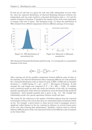
34. Chapter 3. Matching iris codes 3.2. Performance of the code
The implications of performing the orientation correction for uncorrelated iris pro-
vides a new skewed distribution with a reduced mean as shown in fig. 3.4.
In practice, the resultant distribution after seeking the best match between [−5, 5]◦
orientations, accounting for a total of n = 11 different trials:
Figure 3.3: Original HD distribution Figure 3.4: Rotated HD distribution
Since only the smallest value in each group of n = 11 samples was retained, the new
distribution is skewed and biased to a lower mean value HD= 0.4702, as we would
expected from the theory of extreme value sampling.
3.2 Performance of the code
A primary question is whether there is independent variation in iris detail, both
within a given iris and across the human population. Any systematic correlations
in iris detail across the population or within itself would reduce its entropy, which
means that some bits in the code would become irrelevant. From the principle of
entropy we know that a code of any length has maximum information capacity if
all its possible states are equiprobable. However it doesn’t mean that all these bits
are of interest since there would be present information bits as well as noisy bits.
Further development of this project should address this problem by discerning which
are the bits of information and how to retain them while suppressing the most part
of noisy bits (compacting the code).
25

35. Chapter 4
Experimental results
The Image Database of study in this project was CASIA Iris Version 1 collected by
the Chinese Academy of Sciences [13] which includes 756 iris images from 108 eyes
being all left eyes. For each one 7 samples are captured with a resolution of 320 pixels
width and 280 in height, by using eight 850 nm NIR illuminators circularly arranged
around the sensor to make sure that iris is uniformly and adequately illuminated.
When comparing different iris codes, the total number of comparisons can be ex-
pressed as N = 756 eyes arranged in groups of k = 2. Thereby, the the total number
of comparisons is:
Ncomparisons =
N
k
=
756
2
= 285390. (4.1)
The total number of inter-class (same eyes) comparisons is the number of eyes times
the number of samples for each eye (Ns) arranged in groups of 2:
Ninter−class = Neyes ×
Ns
k
= 108 ×
7
2
= 2268. (4.2)
The total number of intra-class comparisons can therefore be expressed as:
Nintra−class = Ncomparisons − Ninter−class = 283122. (4.3)
The reason for which this database was chosen is that it was comprised of a reason-
able amount of samples with close eye views providing thereby high radial resolution
of the eyes. The resolution provided that the number of iterations for performing the
segmentation of the iris was reduced when comparing with higher resolution systems
for whom a coarse-to-fine downscaling to upscaling process should be considered to
improve the speed of the segmentation.
26

36. Chapter 4. Experimental results 4.1. Database characterization
4.1 Database characterization
Before addressing the performance of the system it is important to characterize the
performance of the iris segmentation to find out if the results obtained stay consistent
with the anatomic description of the human eye. The first topic to address is about
the non-concentricity of pupil and limbus center. After experimental analysis the
Integro-Differential operator defined in section 2.2 was optimized by setting the
searching region between [−8, 8] both for x and y axis. The following figures depict
the obtained distribution of shifts for the mentioned parameters:
Figure 4.1: Distribution of shifts for x
axis
Figure 4.2: Distribution of shifts for y
axis
From the distribution observed in x axis we can conclude that the samples of study
were composed of left eyes. The reason for this is that by anatomy the pupil center
is shifted towards the nasal region therefore we are seeing a shift towards the left.
Examining the distribution of centers in the y axis we can say that there is no
predisposition of the limbus in being below or above the pupil center. The next step
is to analyze the statistical distance between the pupil and iris center, fig. 4.3 shows
the relative deviation from the limbus center relative to the pupil radius.
Figure 4.3: Distance from limbic center relative to pupil radius
We can see that in most cases the limbus and the pupil are not concentric and that
most of the deviation is comprised within 20% pupil deviation staying therefore,
27

37. Chapter 4. Experimental results 4.1. Database characterization
consistent with the anatomical definitions. After experimental analysis the Integro-
Differential operator was set to search for a range of radius comprised in the interval
r−limbus ∈ [80, 120], and the circular Hough transform was set to search in a range
comprised between rpupil ∈ [20, 70]. The observed distribution along the pupil radius
presented a general concentration in the range [35, 65]. The observed distribution of
radius for the limbus is mainly concentrated in between [100, 115], since the limbus
has a fixed size and its average is consistent among the population its variation can
be understood as the variance in the sampling conditions being this conditioned by
the zoom and distance to the sensor.
Figure 4.4: Distribution of pupil radius Figure 4.5: Distribution of limbus radius
In order to quantify pupil dilation, the ratio between the pupil and limbus radii
is used, such distribution is shown in fig. 4.6. Since large differences in the dila-
tion ratio can harm considerably the performance of the matching procedure it is
important to pay special attention to this parameter.
Figure 4.6: Distribution of dilation ratios (ρ)
Anatomically, a healthy pupil could in principle vary between 0.15 (highly con-
stricted pupil) and 0.75 (highly dilated pupil), the range of values obtained for the
database used is mainly composed from about 0.3 to 0.55 which can be considered
quite stable. Based on the distribution of ρ, images can be divided into three cate-
gories: constricted images (ρ < 0.35) depicted in red, images with a normal dilation
ratio (0.35 ≥ ρ ≤ 0.475) depicted in blue, and dilated images depicted in yellow
28

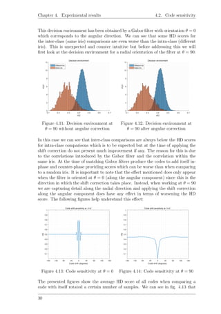
38. Chapter 4. Experimental results 4.2. Code sensitivity
(ρ > 0.475). According to this categorization, the database is mainly composed of
pupils with a normal dilation ratio. This is due to the image acquisition process.
Finally, it is important to characterize the distribution of shifts to apply a proper and
not excessive correction. For this purpose a statistical test was carried to evaluate
the distribution of shifts along the database both for uncorrelated and for the same
iris, such distributions can be seen on fig. 4.7 and 4.8 respectively. This allowed to
understand how where the shifts distributed and to narrow the shift correction to
avoid excessive rotations that would harm the recognition. As the shift distribution
seen on fig. 4.8 shows, the most part of the iris were corrected after applying a shift
correction along the [−5, 5] range accounting for a total of n = 11 corrections.
Figure 4.7: Code shift distribution of
uncorrelated iris
Figure 4.8: Code shift distribution of
same iris
4.2 Code sensitivity
When the shift correction takes place it is interesting to understand how much does
it improve the performance of the recognition. For this reason we will take a look
at the decision environment before and after applying the shift correction:
Figure 4.9: Decision environment at
θ = 0 without angular correction
Figure 4.10: Decision environment at
θ = 0 after angular correction
29

39. Chapter 4. Experimental results 4.2. Code sensitivity
This decision environment has been obtained by a Gabor filter with orientation θ = 0
which corresponds to the angular direction. We can see that some HD scores for
the inter-class (same iris) comparisons are even worse than the intra-class (different
iris). This is unexpected and counter intuitive but before addressing this we will
first look at the decision environment for a radial orientation of the filter at θ = 90:
Figure 4.11: Decision environment at
θ = 90 without angular correction
Figure 4.12: Decision environment at
θ = 90 after angular correction
In this case we can see that inter-class comparisons are always below the HD scores
for intra-class comparisons which is to be expected but at the time of applying the
shift correction do not present much improvement if any. The reason for this is due
to the correlations introduced by the Gabor filter and the correlation within the
same iris. At the time of matching Gabor filters produce the codes to add itself in-
phase and counter-phase providing scores which can be worse than when comparing
to a random iris. It is important to note that the effect mentioned does only appear
when the filter is oriented at θ = 0 (along the angular component) since this is the
direction in which the shift correction takes place. Instead, when working at θ = 90
we are capturing detail along the radial direction and applying the shift correction
along the angular component does have any effect in terms of worsening the HD
score. The following figures help understand this effect:
-180 -135 -90 -45 0 45 90 135 180
Code shift (degrees)
0.1
0.2
0.3
0.4
0.5
0.6
0.7
0.8
0.9
1
HD
Code shift sensitivity at θ=0°
Figure 4.13: Code sensitivity at θ = 0
-180 -135 -90 -45 0 45 90 135 180
Code shift (degrees)
0.1
0.2
0.3
0.4
0.5
0.6
0.7
0.8
0.9
1
HD
Code shift sensitivity at θ=0°
Figure 4.14: Code sensitivity at θ = 90
The presented figures show the average HD score of all codes when comparing a
code with itself rotated a certain number of samples. We can see in fig. 4.13 that
30

40. Chapter 4. Experimental results 4.2. Code sensitivity
we can shift a code in in such a way that its HD score is worse than average whilst
in fig. 4.14 there is no such effect and has a higher tolerance when comparing a
code with a shifted version of itself. This demonstrates why when applying the shift
correction at θ = 90 we could not notice much difference.
31

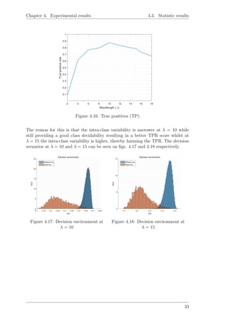
41. Chapter 4. Experimental results 4.3. Statistic results
4.3 Statistic results
To compute the iris code there are many possible Gabor filters which can be used, in
this project the orientation chosen was θ = 0 since it reveals all the radial texture on
the iris and thus provides more discriminant information; the phase offset was set to
φ = 0; the aspect ratio was set to α/β = 1 and finally the wavelength, to optimize
this parameter the “decidability” criteria was chosen since it gives a measure of how
well separated the two distributions are. The “decidability” (d ) criteria is defined
as:
d =
|µ1 − µ2|
σ2
1+σ2
2
2
(4.4)
This measure of decidability is independent of how liberal or conservative is the
acceptance threshold used. Rather, by measuring separation, it reflects the degree
to which any improvement in (say) the false match error rate must be paid for by
a worsening of the failure-to-match error rate. The performance of any biometric
technology can be calibrated by its score, among other metrics. In fig. 4.15 we can
see the decidability obtained for every wavelength when a shift correction between
[−5, 5]◦
was applied.
2 4 6 8 10 12 14 16 18
Wavelength ( λ)
0
0.5
1
1.5
2
2.5
3
3.5
4
4.5
Decidability(d′
)
Figure 4.15: Decidability
As we can see in fig. 4.15 the best decidability is obtained at λ = 15. While it is
important to characterize the decidability of the system it is not the only important
aspect to take into consideration, there may exist other wavelengths for which the
decidability criteria may not be optimum but provide better decision environments
according to a certain criteria, for this reason we considered the study of the “true
positive ratio” (TPR) as a measure of how well the system can identify an individual
without making any false decisions, such a plot can be seen in fig. 4.16; according
to this graphic, the best decision environment when considering the highest possible
TPR is achieved at λ = 10 with TPR= 0.87 whilst at λ = 15 the TPR= 0.79.
32

42. Chapter 4. Experimental results 4.3. Statistic results
2 4 6 8 10 12 14 16 18
Wavelength ( λ)
0.1
0.2
0.3
0.4
0.5
0.6
0.7
0.8
0.9
1
Truepositiverate
Figure 4.16: True positives (TP)
The reason for this is that the intra-class variability is narrower at λ = 10 while
still providing a good class decidability resulting in a better TPR score whilst at
λ = 15 the intra-class variability is higher, thereby harming the TPR. The decision
scenarios at λ = 10 and λ = 15 can be seen on figs. 4.17 and 4.18 respectively.
Figure 4.17: Decision environment at
λ = 10
Figure 4.18: Decision environment at
λ = 15
33

43. Chapter 5
Conclusions and future work
After the realization of the project we have the theoretical basis and a first approach
to an iris biometric system adapted to the NIR spectrum. The system extracts an iris
code generated from the segmentation of the iris which allows the system to match
with other stored codes by means of the bitwise operator XOR which provides an
amazing speed when matching iris codes since the XOR operator can be executed in
a single instruction in the processor. The system relies on a proper segmentation of
the iris which can in some cases become quite tricky. It is very important to capture
as much details of the iris as possible and in this project a single optimized Gabor
filter was chosen but further development of the texture analysis should introduce
modifications in the Gabor filter according to the region of study to address the
heterogeneous structure of the iris. Further development of the system may also
include segmentation of the eyelashes, eyelids and shadows (EES) minimizing as
much as possible the suppression of texture information. Also a proper detailed
study of the intrinsic correlations in the iris should be done compacting the generated
code.
Future adaptations of the system may also be capable to operate on the visible
spectrum. Working on the VW spectrum has the additional difficulty that reflections
should be addressed when segmenting the iris. Furthermore, it would be interesting
to combine facial recognition algorithms to extract iris codes.
34

44. Bibliography
[1] J. Daugman, “How iris recognition works,” Circuits and Systems for Video
Technology, IEEE Transactions on, vol. 14, no. 1, pp. 21–30, 2004.
[2] J. R. Charlier, M. Behague, and C. Buquet, “Shift of pupil center with pupil
constriction.”
[3] B. Green, “Canny edge detection algorithm,” pp. 1–7, 2002. [Online]. Available:
http://dasl.mem.drexel.edu/alumni/bGreen/www.pages.drexel.edu/ weg22/can tut.html
[4] J. Canny, “A Computational Approach to Edge Detection,” IEEE Transactions
on Pattern Analysis and Machine Intelligence, vol. PAMI-8, no. 6, pp. 679–698,
1986.
[5] A. Basit, M. Y. Javed, and M. A. Anjum, “Eyelid detection in localized iris
images,” Proceedings - 2nd International Conference on Emerging Technologies
2006, ICET 2006, no. November, pp. 157–159, 2006.
[6] T. H. Min and R. H. Park, “Comparison of eyelid and eyelash detection algo-
rithms for performance improvement of iris recognition,” Proceedings - Inter-
national Conference on Image Processing, ICIP, pp. 257–260, 2008.
[7] T. Wang, M. Han, and H. Wan, “Improved and robust eyelash and eyelid
location method,” 2012 International Conference on Wireless Communications
and Signal Processing, WCSP 2012, 2012.
[8] C. Academy and P. O. Box, “Enhanced Usability Of Iris Recognition Via Ef-
ficient User Interface And Iris Image Restoration Zhaofeng He , Zhenan Sun
, Tieniu Tan and Xianchao Qiu Center for Biometrics and Security Research
National Laboratory of Pattern Recognition , Institute of Aut,” Security, pp.
261–264, 2008.
[9] L. Yang, Y. X. Dong, Z. T. Wu, and C. Engineering, “[ J [ J,” vol. 1, no.
Iccda, pp. 533–536, 2010.
[10] I. Tomeo-Reyes, A. Ross, A. D. Clark, and V. Chandran, “A biomechanical
approach to iris normalization,” Proceedings of 2015 International Conference
on Biometrics, ICB 2015, pp. 9–16, 2015.
[11] Z. Lin and B. Lu, “Iris recognition method based on the optimized Gabor
filters,” Image and Signal Processing (CISP), 2010 3rd International Congress
on, vol. 4, no. 1, pp. 1868–1872, 2010.
35

45. Bibliography Bibliography
[12] J. G. Daugman, “Complete Discrete 2-D Gabor Transforms by Neural Networks
for Image Analysis and Compression,” IEEE Transactions on Acoustics, Speech,
and Signal Processing, vol. 36, no. 7, pp. 1169–1179, 1988.
[13] Note on CASIA-Iris V1, “Chinese Academy of Sciences Institute of Automation
(CASIA).” [Online]. Available: http://biometrics.idealtest.org/
[14] P. Podder, T. Z. Khan, M. H. Khan, and M. M. Rahman, “An Efficient Iris Seg-
mentation Model Based on Eyelids and Eyelashes Detection in Iris Recognition
System,” 2015.
36