HLM: Hierarchical Linear Modeling Katy Pearce, CRRC Armenia,  May 15-16, 2008
Introduction Katy Pearce, current PhD student in Communication at University of California, Santa Barbara. Communication is sociology + psychology. Studies technology and how cultural characteristics can moderate technology adoption, attitudes, and use.
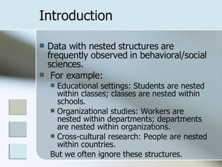
Introduction Data with nested structures are frequently observed in behavioral/social sciences. For example: Educational settings: Students are nested within classes; classes are nested within schools. Organizational studies: Workers are nested within departments; departments are nested within organizations. Cross-cultural research: People are nested within countries. But we often ignore these structures.
Example 1 Educational achievement: Imagine 5 little boys who are very similar: parental education is the same = low, parental income is the same = low, IQ is the same = low, etc. These 5 boys go to 5 different schools: an excellent school, a very good school, a good school, a poor school, and a very poor school. With HLM we can compare the impact of these different types of schools on the boys’ education achievement (test scores, grades, etc.). One can imagine that the mean parental education, parental income, and IQ are low are the very poor school and are high at the excellent school.  With HLM we can control for variance at both the individual and the mean level.
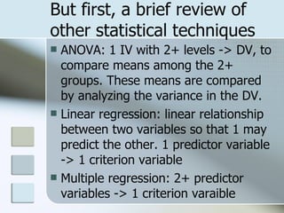
But first, a brief review of other statistical techniques ANOVA: 1 IV with 2+ levels -> DV, to compare means among the 2+ groups. These means are compared by analyzing the variance in the DV.  Linear regression: linear relationship between two variables so that 1 may predict the other. 1 predictor variable -> 1 criterion variable Multiple regression: 2+ predictor variables -> 1 criterion varaible
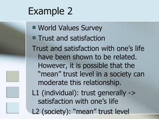
Example 2 World Values Survey Trust and satisfaction Trust and satisfaction with one’s life have been shown to be related. However, it is possible that the “mean” trust level in a society can moderate this relationship. L1 (individual): trust generally -> satisfaction with one’s life L2 (society): “mean” trust level
First, we need to get the data ready Step 1: prepare the file The World Values Survey is too big for the student version of HLM, so let’s take ~10% of the sample and save the file. Sort by nation [v2], save the file. Aggregate the data: “break variable” is nation [v2] and “aggregate variables” are life satisfaction [v81] and  take advantage [v26], but sure to create a new data file
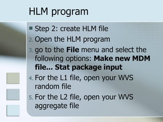
HLM program Step 2: create HLM file Open the HLM program go to the  File  menu and select the following options:  Make new MDM file... Stat package input For the L1 file, open your WVS random file For the L2 file, open your WVS aggregate file
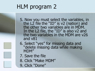
HLM program 2 5. Now you must select the variables, in the L2 file the “ID” is v2 (nation) and the other two variables are in MDM. In the L2 file, the “ID” is also v2 and the two variables in the MDM are v26 and v81 6. Select “yes” for missing data and “delete missing data while making MDM” 7. Save the file 8. Click “Make MDM” 9. Click “Done”
Effects Before we get to the actual data analysis, let’s talk about effects in HLM. Fixed effects  are the only levels of a variable in which a researcher is interested in studying.  Random effects  are a subset of the total possible levels of a variable where the researcher is interested in generalizing to levels not observed. For example, let’s say that we set up a school where in different classrooms, some of the students receive special tutoring and others are in a control group. A  fixed effect variable  would be which group the student was in: control or treatment, only two groups exist.  A  random effect variable  would be the classroom that the student was in, as it shouldn’t matter to the study.
HLM analysis – Means as Outcomes 9. Let’s start with specifying the L1 model. First we need to tell the program what our DV is, life satisfaction or [v81]. Click on v81 and select “outcome variable.”  10. Now we need to tell the program what our fixed and random effects are. V26 (trust) is a fixed effect, because we care about it. The intercept and slope are by default random effects. 11. Repeat for L2. 12. Click “Run analysis”
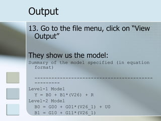
Output 13. Go to the file menu, click on “View Output” They show us the model: Summary of the model specified (in equation format) --------------------------------------------------- Level-1 Model Y = B0 + B1*(V26) + R Level-2 Model B0 = G00 + G01*(V26_1) + U0 B1 = G10 + G11*(V26_1)
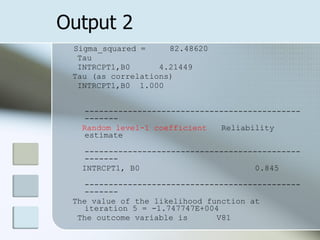
Output 2 Sigma_squared =  82.48620 Tau INTRCPT1,B0  4.21449  Tau (as correlations) INTRCPT1,B0  1.000 ---------------------------------------------------- Random level-1 coefficient  Reliability estimate ---------------------------------------------------- INTRCPT1, B0  0.845 ---------------------------------------------------- The value of the likelihood function at iteration 5 = -1.747747E+004 The outcome variable is  V81
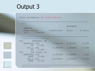
Output 3 Final estimation of  fixed effects : --------------------------------------------------------- Standard  Approx. Fixed Effect  Coefficient  Error  T-ratio  d.f.  P-value ---------------------------------------------------------------------------- For  INTRCPT1, B0 INTRCPT2, G00  7.652744  0.870587  8.790  38  0.000 V26_1, G01  -0.440045  0.404599  -1.088  38  0.284 For  V26 slope, B1 INTRCPT2, G10  0.333436  0.195697  1.704  4806  0.088 V26_1, G11  -0.070027  0.078756  -0.889  4806  0.374 ----------------------------------------------------------------------------
Output 4 The outcome variable is  V81 Final estimation of  fixed effects (with robust standard errors) ---------------------------------------------------------------------------- Standard  Approx. Fixed Effect  Coefficient  Error  T-ratio  d.f.  P-value ---------------------------------------------------------------------------- For  INTRCPT1, B0 INTRCPT2, G00  7.652744  0.670477  11.414  38  0.000 V26_1, G01  -0.440045  0.309190  -1.423  38  0.163 For  V26 slope, B1 INTRCPT2, G10  0.333436  0.212963  1.566  4806  0.117 V26_1, G11  -0.070027  0.075376  -0.929  4806  0.353 ----------------------------------------------------------------------------
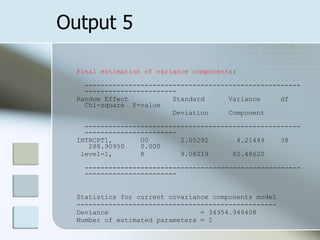
Output 5 Final estimation of variance components : ----------------------------------------------------------------------------- Random Effect  Standard  Variance  df  Chi-square  P-value Deviation  Component ----------------------------------------------------------------------------- INTRCPT1,  U0  2.05292  4.21449  38  288.90950  0.000 level-1,  R  9.08219  82.48620 ----------------------------------------------------------------------------- Statistics for current covariance components model -------------------------------------------------- Deviance  = 34954.948408 Number of estimated parameters = 2
What to do with this output? First,  we must calculate the intraclass correlation. ρ  =  τ 00  / ( τ 00  +  σ 2 )  4.21449 / (4.21449 + 82.48620) = 4.21449/   86.70069 = 0.0486096477 Which means that ~5% of the variance is at the national level (L2), and that 95% of the variance is at the individual (L1) level.
Let’s try some different WVS examples Family important [v4] -> Work important [v8] ~6% of variance is at the national level. Democracy isn’t good [v171] -> Having army rule [v166] ~57% of the variance is at the national level.
CRRC DI 3 countries (AM, AZ, and GE) are technically too small of groups to compare, but can compare regions First, Armenia only, sort by quadrant. What variables would differ by quadrant? English language knowledge level [e9_2] -> political cooperation with U.S. [p15_6] 3% of variance is at the quadrant level
Your own data Your own data set Needs to have 10+ groups Continuous variables or categorical, but preferably with a larger scale If you don’t have your own data, you’re welcome to use the WVS or CRRC DI  or  if there is a topic that you’re interested in, get a data set before tomorrow or give me a sense of your interests and I’ll find one.
Other datasets freely available http://www.icpsr.umich.edu/ : archive of thousands of datasets http://unstats.un.org/unsd/default.htm : United Nations Statistics http://www.worldbank.org/data  : World Bank data

Hierarchical Linear Modeling

  • 1.
    HLM: Hierarchical LinearModeling Katy Pearce, CRRC Armenia, May 15-16, 2008
  • 2.
    Introduction Katy Pearce,current PhD student in Communication at University of California, Santa Barbara. Communication is sociology + psychology. Studies technology and how cultural characteristics can moderate technology adoption, attitudes, and use.
  • 3.
    Introduction Data withnested structures are frequently observed in behavioral/social sciences. For example: Educational settings: Students are nested within classes; classes are nested within schools. Organizational studies: Workers are nested within departments; departments are nested within organizations. Cross-cultural research: People are nested within countries. But we often ignore these structures.
  • 4.
    Example 1 Educationalachievement: Imagine 5 little boys who are very similar: parental education is the same = low, parental income is the same = low, IQ is the same = low, etc. These 5 boys go to 5 different schools: an excellent school, a very good school, a good school, a poor school, and a very poor school. With HLM we can compare the impact of these different types of schools on the boys’ education achievement (test scores, grades, etc.). One can imagine that the mean parental education, parental income, and IQ are low are the very poor school and are high at the excellent school. With HLM we can control for variance at both the individual and the mean level.
  • 5.
    But first, abrief review of other statistical techniques ANOVA: 1 IV with 2+ levels -> DV, to compare means among the 2+ groups. These means are compared by analyzing the variance in the DV. Linear regression: linear relationship between two variables so that 1 may predict the other. 1 predictor variable -> 1 criterion variable Multiple regression: 2+ predictor variables -> 1 criterion varaible
  • 6.
    Example 2 WorldValues Survey Trust and satisfaction Trust and satisfaction with one’s life have been shown to be related. However, it is possible that the “mean” trust level in a society can moderate this relationship. L1 (individual): trust generally -> satisfaction with one’s life L2 (society): “mean” trust level
  • 7.
    First, we needto get the data ready Step 1: prepare the file The World Values Survey is too big for the student version of HLM, so let’s take ~10% of the sample and save the file. Sort by nation [v2], save the file. Aggregate the data: “break variable” is nation [v2] and “aggregate variables” are life satisfaction [v81] and take advantage [v26], but sure to create a new data file
  • 8.
    HLM program Step2: create HLM file Open the HLM program go to the File menu and select the following options: Make new MDM file... Stat package input For the L1 file, open your WVS random file For the L2 file, open your WVS aggregate file
  • 9.
    HLM program 25. Now you must select the variables, in the L2 file the “ID” is v2 (nation) and the other two variables are in MDM. In the L2 file, the “ID” is also v2 and the two variables in the MDM are v26 and v81 6. Select “yes” for missing data and “delete missing data while making MDM” 7. Save the file 8. Click “Make MDM” 9. Click “Done”
  • 10.
    Effects Before weget to the actual data analysis, let’s talk about effects in HLM. Fixed effects are the only levels of a variable in which a researcher is interested in studying. Random effects are a subset of the total possible levels of a variable where the researcher is interested in generalizing to levels not observed. For example, let’s say that we set up a school where in different classrooms, some of the students receive special tutoring and others are in a control group. A fixed effect variable would be which group the student was in: control or treatment, only two groups exist. A random effect variable would be the classroom that the student was in, as it shouldn’t matter to the study.
  • 11.
    HLM analysis –Means as Outcomes 9. Let’s start with specifying the L1 model. First we need to tell the program what our DV is, life satisfaction or [v81]. Click on v81 and select “outcome variable.” 10. Now we need to tell the program what our fixed and random effects are. V26 (trust) is a fixed effect, because we care about it. The intercept and slope are by default random effects. 11. Repeat for L2. 12. Click “Run analysis”
  • 12.
    Output 13. Goto the file menu, click on “View Output” They show us the model: Summary of the model specified (in equation format) --------------------------------------------------- Level-1 Model Y = B0 + B1*(V26) + R Level-2 Model B0 = G00 + G01*(V26_1) + U0 B1 = G10 + G11*(V26_1)
  • 13.
    Output 2 Sigma_squared= 82.48620 Tau INTRCPT1,B0 4.21449 Tau (as correlations) INTRCPT1,B0 1.000 ---------------------------------------------------- Random level-1 coefficient Reliability estimate ---------------------------------------------------- INTRCPT1, B0 0.845 ---------------------------------------------------- The value of the likelihood function at iteration 5 = -1.747747E+004 The outcome variable is V81
  • 14.
    Output 3 Finalestimation of fixed effects : --------------------------------------------------------- Standard Approx. Fixed Effect Coefficient Error T-ratio d.f. P-value ---------------------------------------------------------------------------- For INTRCPT1, B0 INTRCPT2, G00 7.652744 0.870587 8.790 38 0.000 V26_1, G01 -0.440045 0.404599 -1.088 38 0.284 For V26 slope, B1 INTRCPT2, G10 0.333436 0.195697 1.704 4806 0.088 V26_1, G11 -0.070027 0.078756 -0.889 4806 0.374 ----------------------------------------------------------------------------
  • 15.
    Output 4 Theoutcome variable is V81 Final estimation of fixed effects (with robust standard errors) ---------------------------------------------------------------------------- Standard Approx. Fixed Effect Coefficient Error T-ratio d.f. P-value ---------------------------------------------------------------------------- For INTRCPT1, B0 INTRCPT2, G00 7.652744 0.670477 11.414 38 0.000 V26_1, G01 -0.440045 0.309190 -1.423 38 0.163 For V26 slope, B1 INTRCPT2, G10 0.333436 0.212963 1.566 4806 0.117 V26_1, G11 -0.070027 0.075376 -0.929 4806 0.353 ----------------------------------------------------------------------------
  • 16.
    Output 5 Finalestimation of variance components : ----------------------------------------------------------------------------- Random Effect Standard Variance df Chi-square P-value Deviation Component ----------------------------------------------------------------------------- INTRCPT1, U0 2.05292 4.21449 38 288.90950 0.000 level-1, R 9.08219 82.48620 ----------------------------------------------------------------------------- Statistics for current covariance components model -------------------------------------------------- Deviance = 34954.948408 Number of estimated parameters = 2
  • 17.
    What to dowith this output? First, we must calculate the intraclass correlation. ρ = τ 00 / ( τ 00 + σ 2 ) 4.21449 / (4.21449 + 82.48620) = 4.21449/ 86.70069 = 0.0486096477 Which means that ~5% of the variance is at the national level (L2), and that 95% of the variance is at the individual (L1) level.
  • 18.
    Let’s try somedifferent WVS examples Family important [v4] -> Work important [v8] ~6% of variance is at the national level. Democracy isn’t good [v171] -> Having army rule [v166] ~57% of the variance is at the national level.
  • 19.
    CRRC DI 3countries (AM, AZ, and GE) are technically too small of groups to compare, but can compare regions First, Armenia only, sort by quadrant. What variables would differ by quadrant? English language knowledge level [e9_2] -> political cooperation with U.S. [p15_6] 3% of variance is at the quadrant level
  • 20.
    Your own dataYour own data set Needs to have 10+ groups Continuous variables or categorical, but preferably with a larger scale If you don’t have your own data, you’re welcome to use the WVS or CRRC DI or if there is a topic that you’re interested in, get a data set before tomorrow or give me a sense of your interests and I’ll find one.
  • 21.
    Other datasets freelyavailable http://www.icpsr.umich.edu/ : archive of thousands of datasets http://unstats.un.org/unsd/default.htm : United Nations Statistics http://www.worldbank.org/data : World Bank data