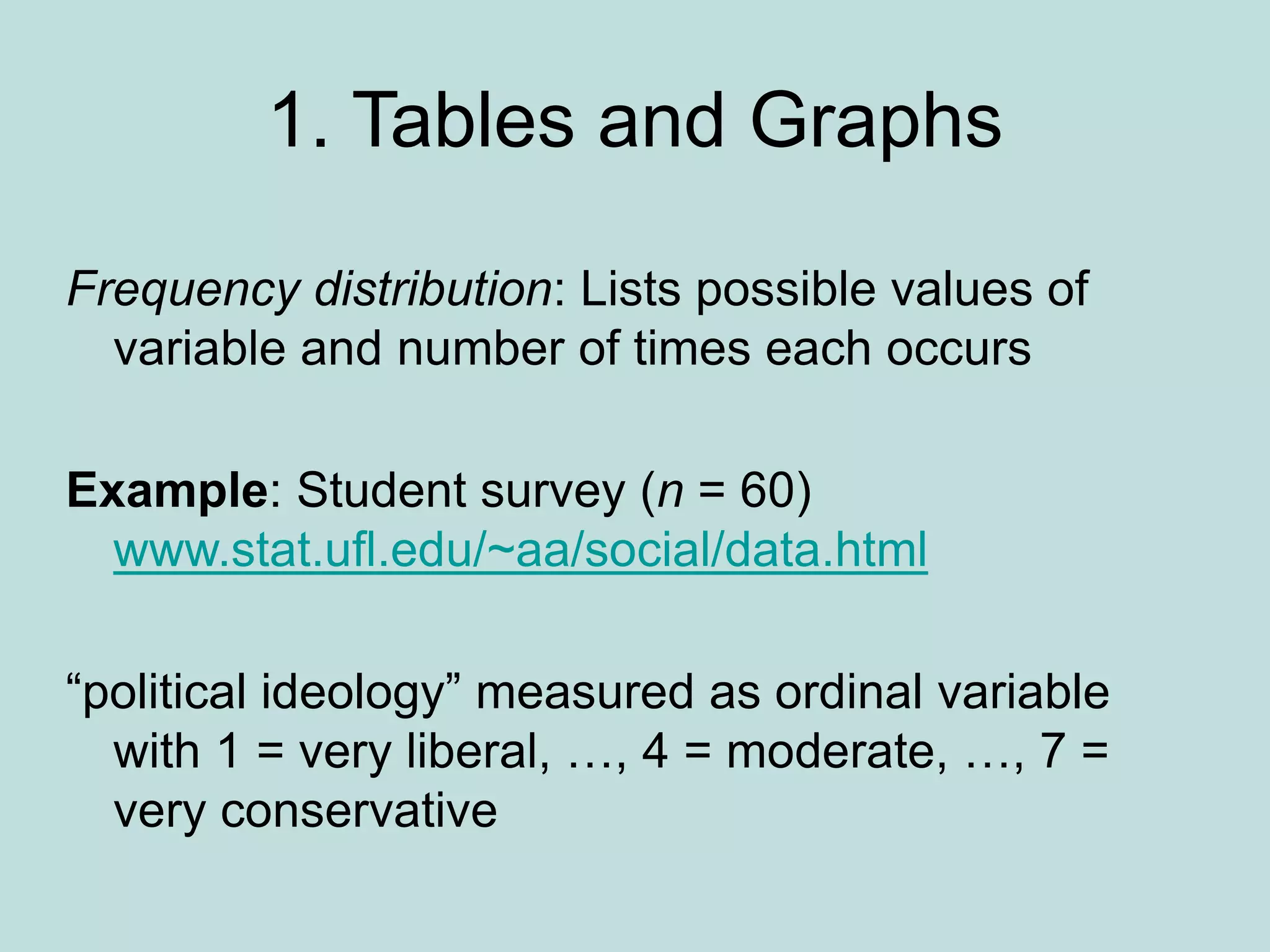
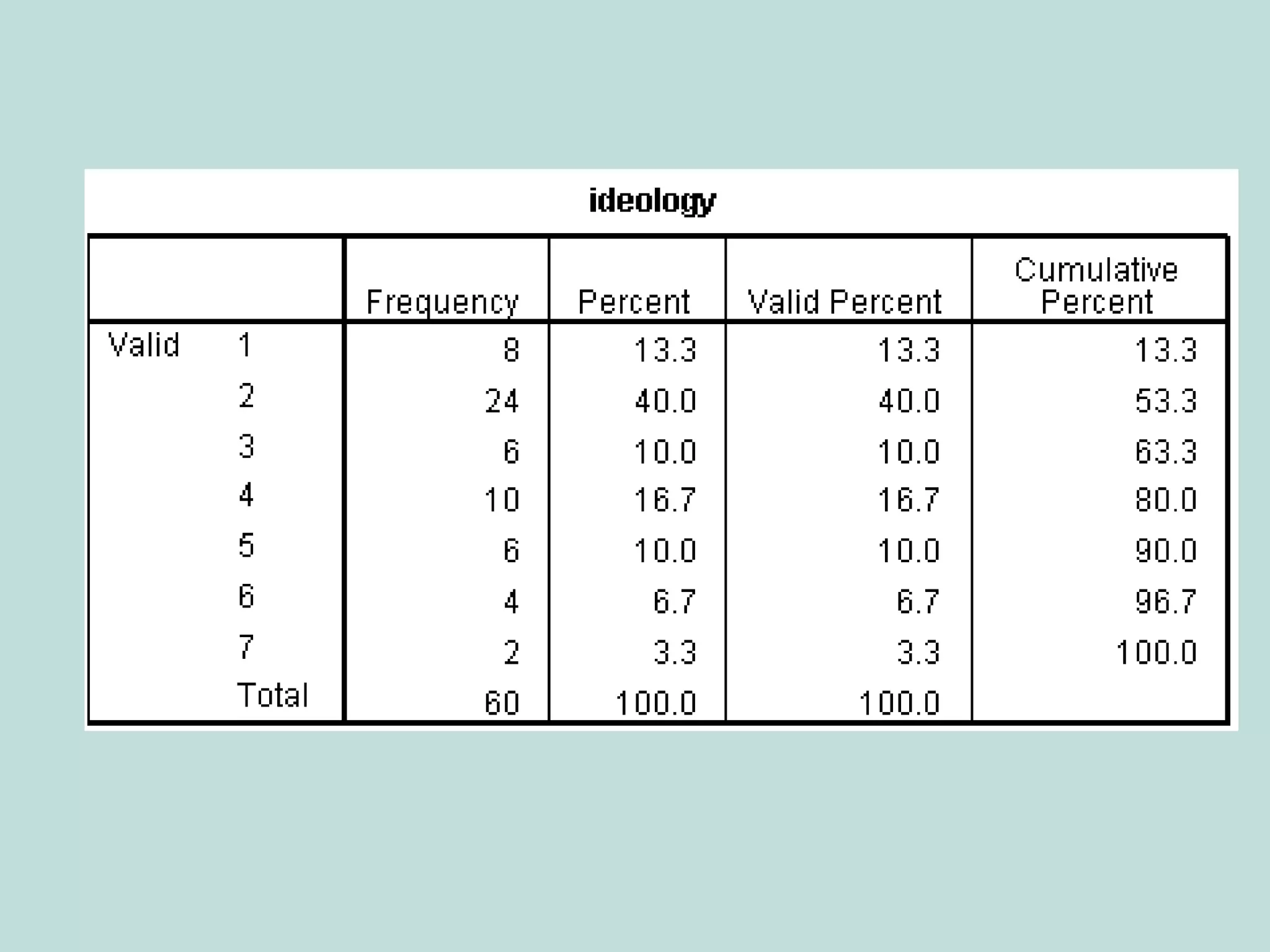
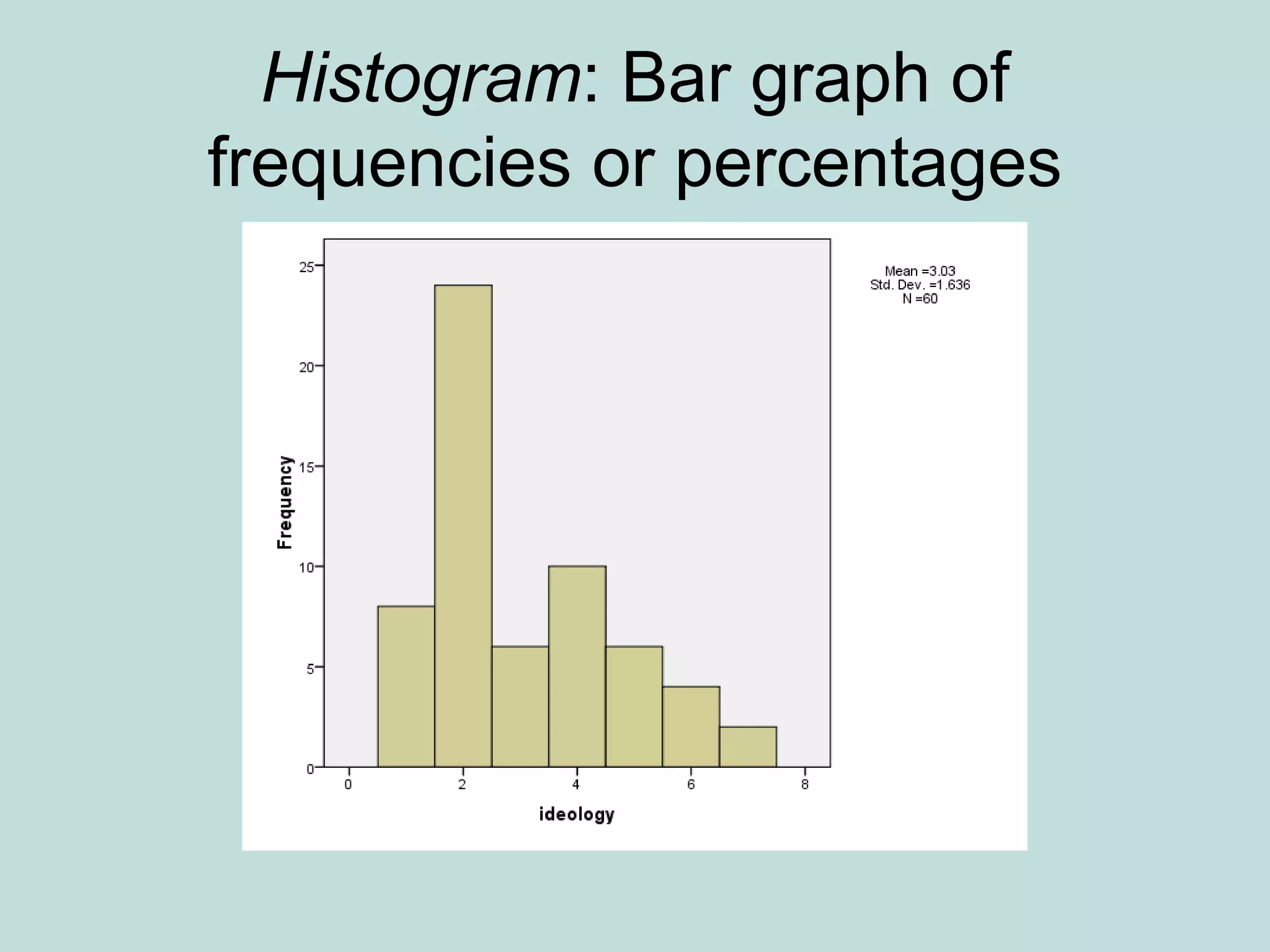
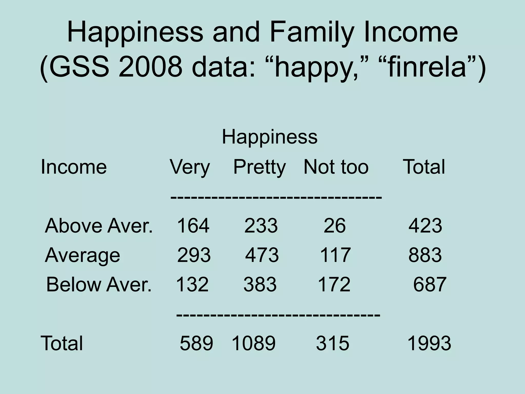
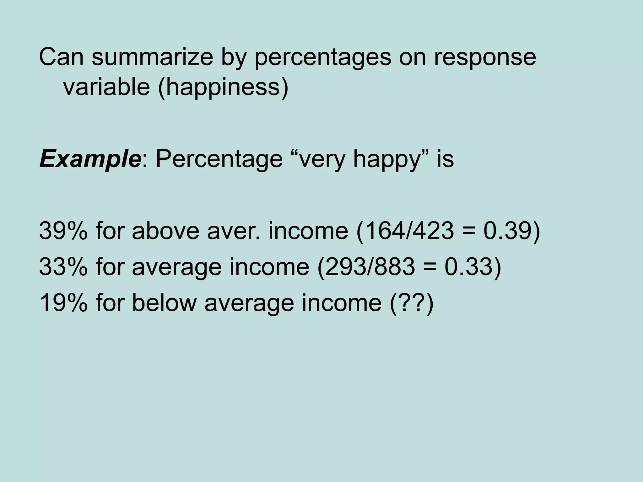
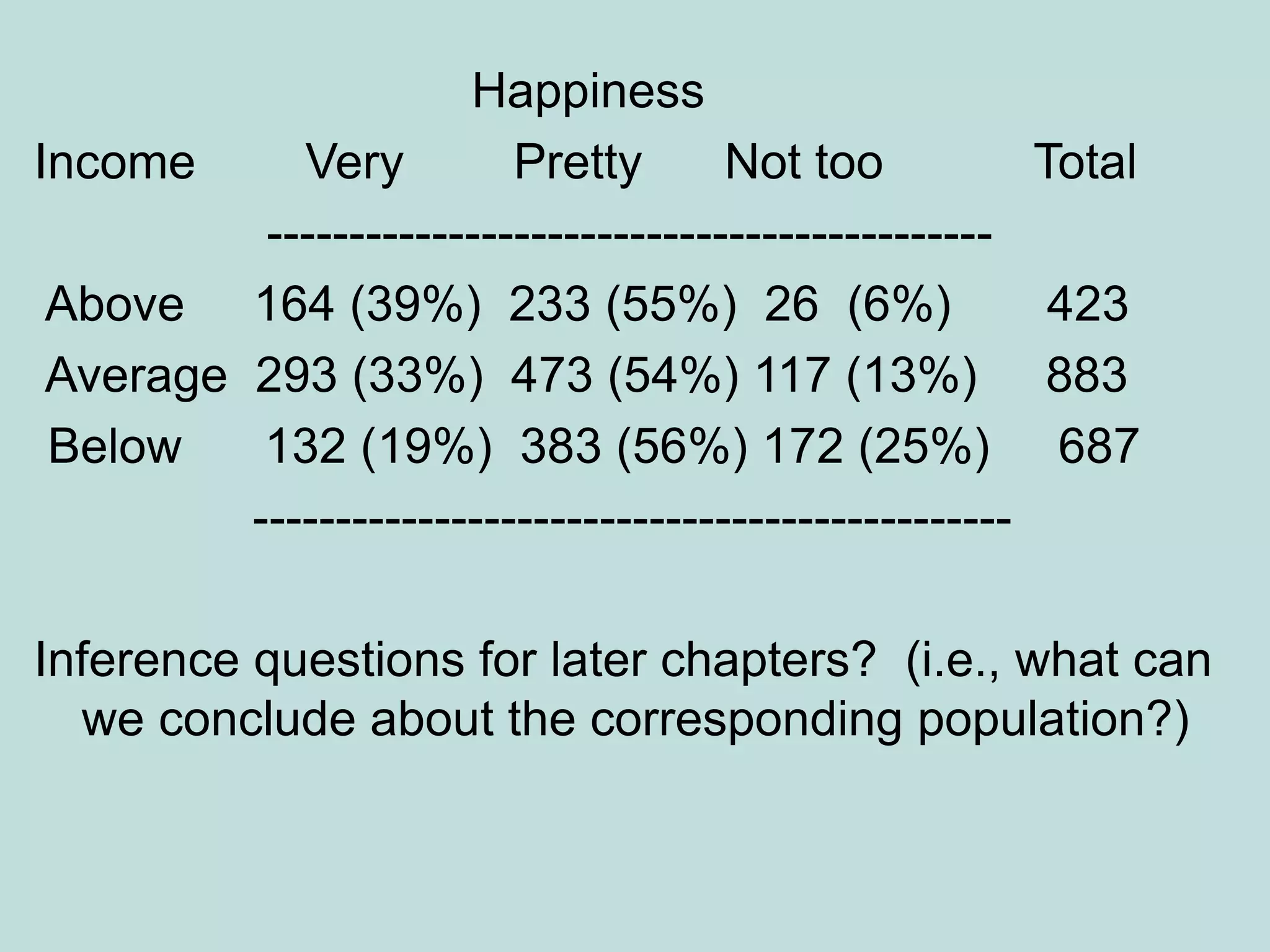
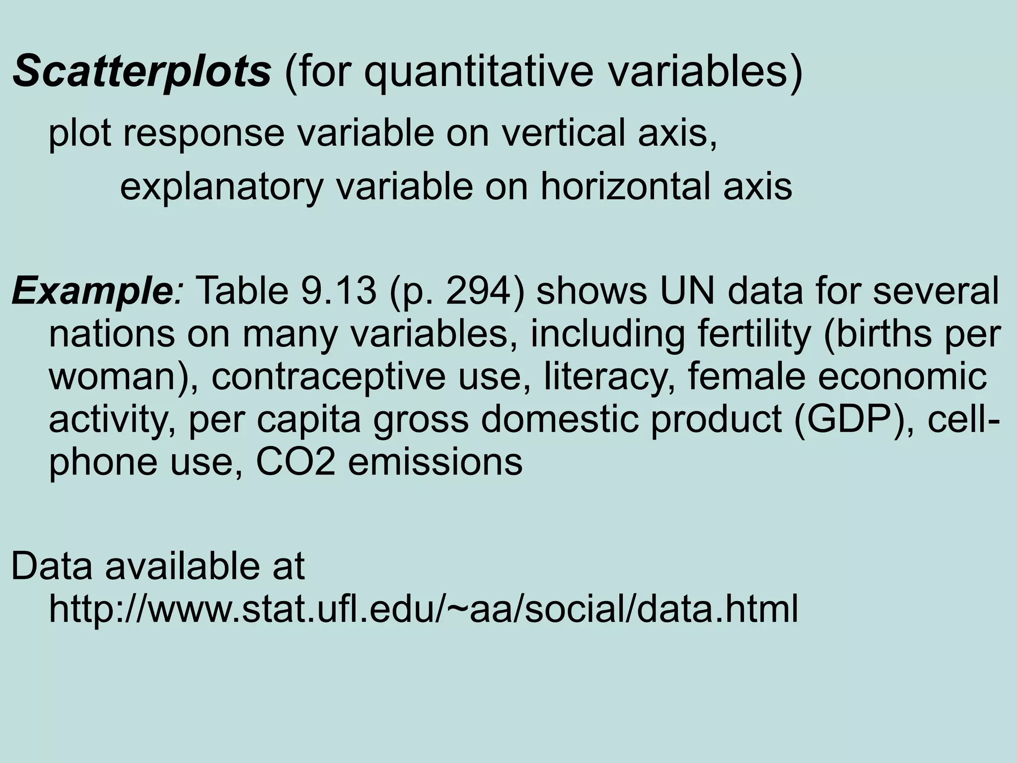
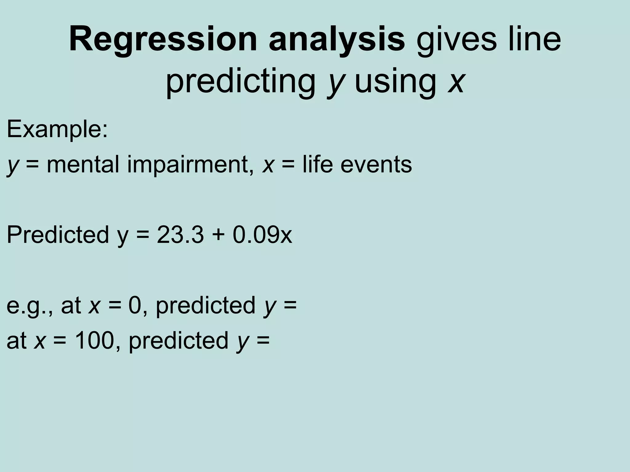
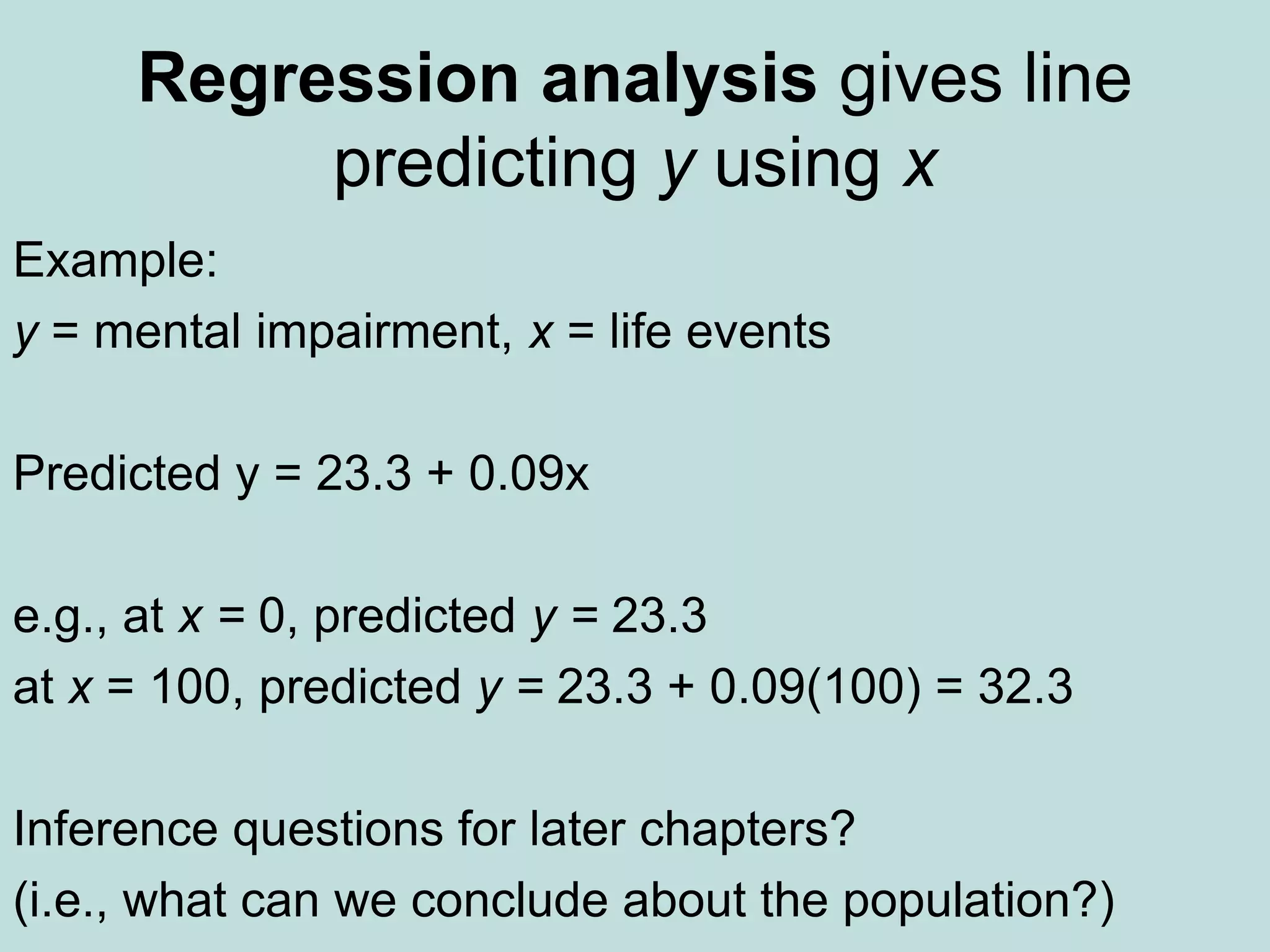
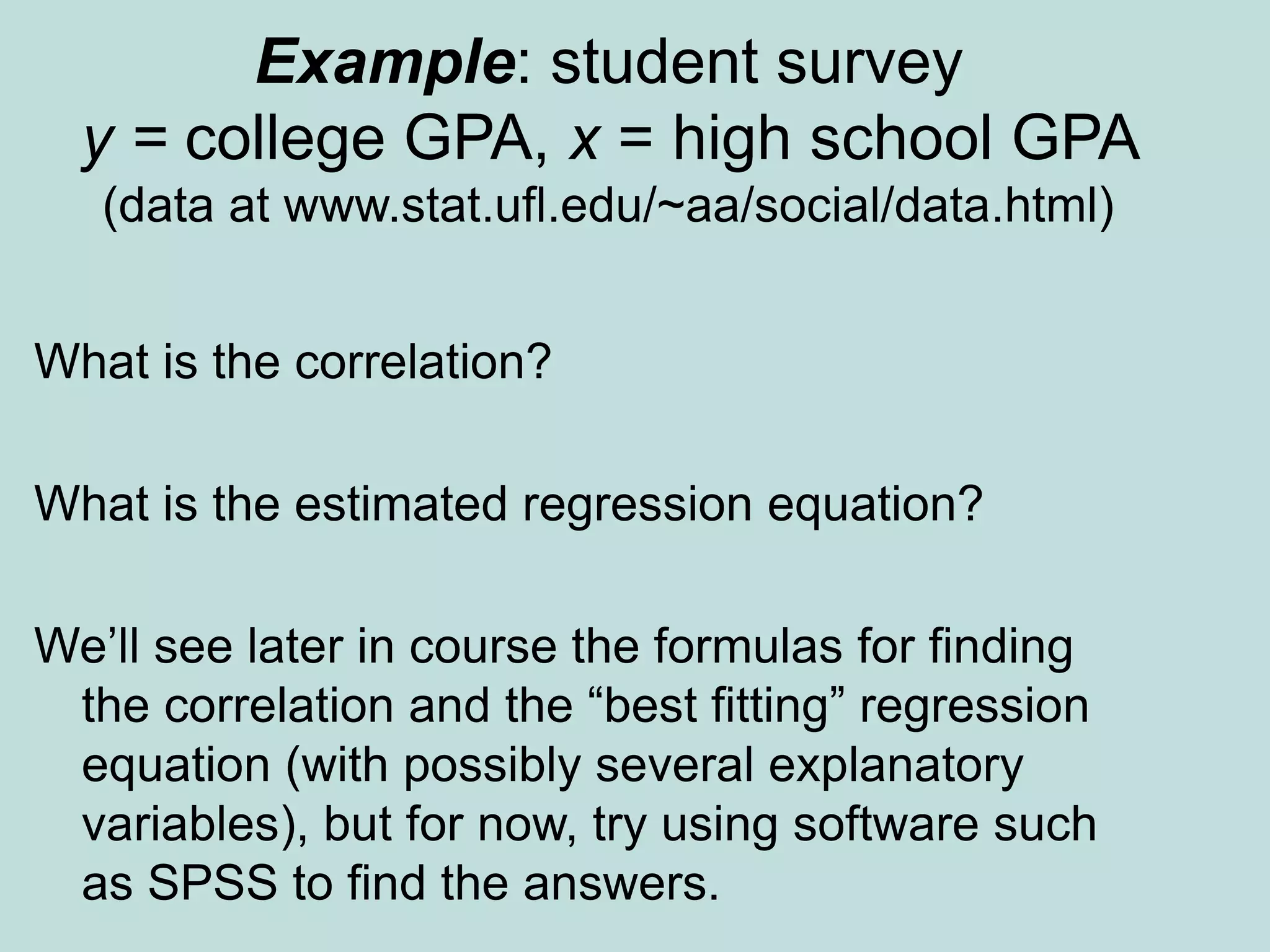
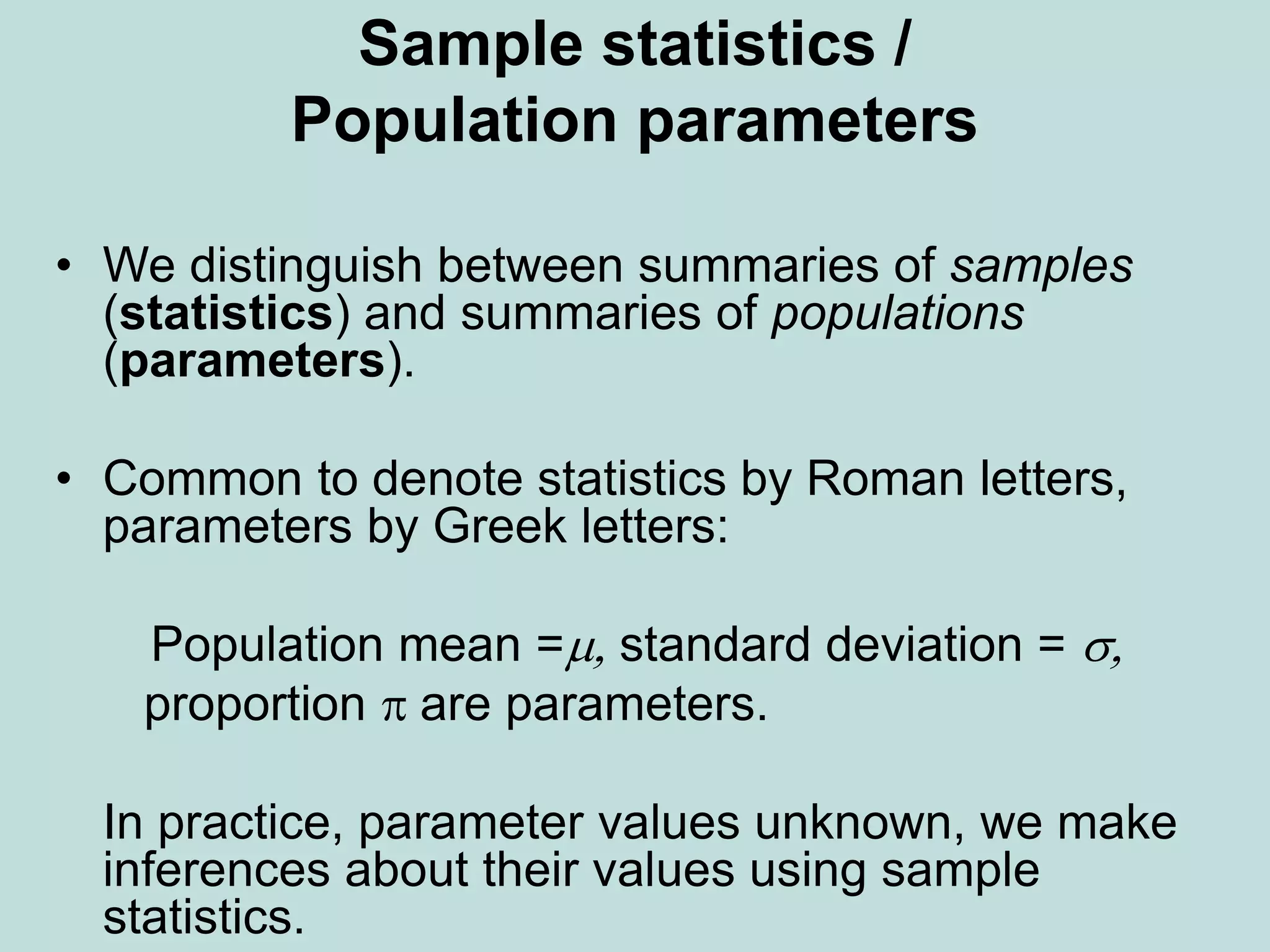
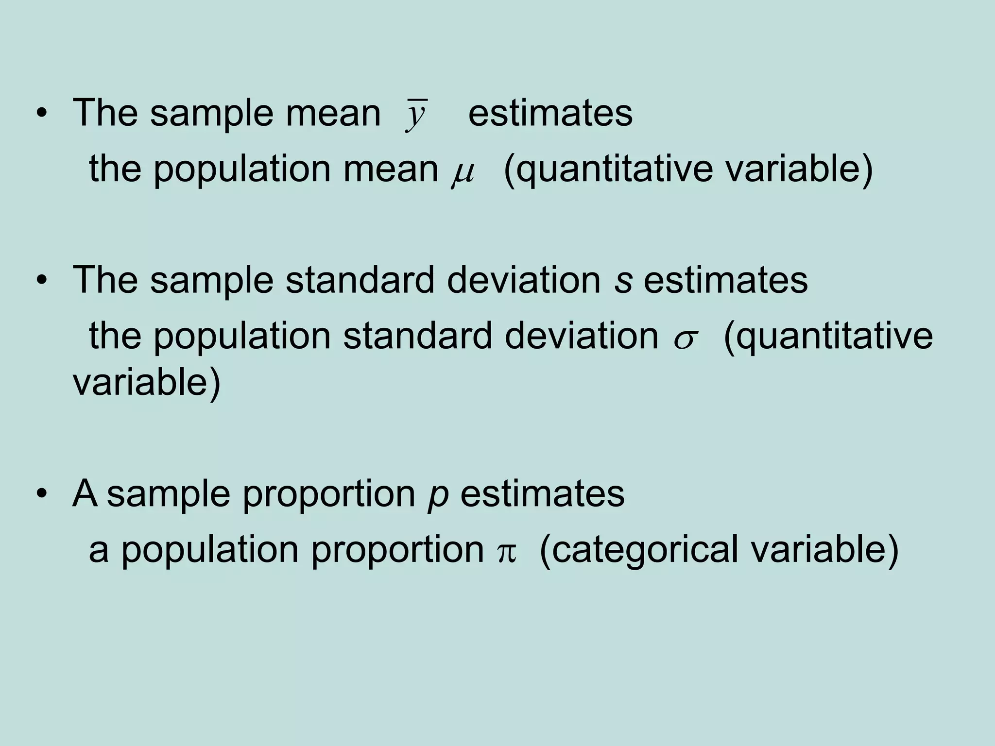
SlideShare a Scribd company logo
1 of 41
3. Descriptive Statistics
• Describing data with tables and graphs
(quantitative or categorical variables)
• Numerical descriptions of center, variability,
position (quantitative variables)
• Bivariate descriptions (In practice, most
studies have several variables)
Frequency distribution: Lists possible values of
variable and number of times each occurs
Example: Student survey (n = 60)
www.stat.ufl.edu/~aa/social/data.html
“political ideology” measured as ordinal variable
with 1 = very liberal, …, 4 = moderate, …, 7 =
very conservative
1. Tables and Graphs
Histogram: Bar graph of
frequencies or percentages
Shapes of histograms
(for quantitative variables)
• Bell-shaped (IQ, SAT, political ideology in all U.S. )
• Skewed right (annual income, no. times arrested)
• Skewed left (score on easy exam)
• Bimodal (polarized opinions)
Ex. GSS data on sex before marriage in Exercise 3.73:
always wrong, almost always wrong, wrong only
sometimes, not wrong at all
category counts 238, 79, 157, 409
Stem-and-leaf plot (John Tukey, 1977)
Example: Exam scores (n = 40 students)
Stem Leaf
3 6
4
5 37
6 235899
7 011346778999
8 00111233568889
9 02238
2.Numerical descriptions
Let y denote a quantitative variable, with
observations y1 , y2 , y3 , … , yn
a. Describing the center
Median: Middle measurement of ordered sample
Mean:
1 2 ... n i
y y y y
y
n n
   
 
Example: Annual per capita carbon dioxide emissions
(metric tons) for n = 8 largest nations in population
size
Bangladesh 0.3, Brazil 1.8, China 2.3, India 1.2,
Indonesia 1.4, Pakistan 0.7, Russia 9.9, U.S. 20.1
Ordered sample:
Median =
Mean =
y
Example: Annual per capita carbon dioxide emissions
(metric tons) for n = 8 largest nations in population
size
Bangladesh 0.3, Brazil 1.8, China 2.3, India 1.2,
Indonesia 1.4, Pakistan 0.7, Russia 9.9, U.S. 20.1
Ordered sample: 0.3, 0.7, 1.2, 1.4, 1.8, 2.3, 9.9, 20.1
Median =
Mean =
y
Example: Annual per capita carbon dioxide emissions
(metric tons) for n = 8 largest nations in population
size
Bangladesh 0.3, Brazil 1.8, China 2.3, India 1.2,
Indonesia 1.4, Pakistan 0.7, Russia 9.9, U.S. 20.1
Ordered sample: 0.3, 0.7, 1.2, 1.4, 1.8, 2.3, 9.9, 20.1
Median = (1.4 + 1.8)/2 = 1.6
Mean = (0.3 + 0.7 + 1.2 + … + 20.1)/8 = 4.7
y
Properties of mean and median
• For symmetric distributions, mean = median
• For skewed distributions, mean is drawn in
direction of longer tail, relative to median
• Mean valid for interval scales, median for
interval or ordinal scales
• Mean sensitive to “outliers” (median often
preferred for highly skewed distributions)
• When distribution symmetric or mildly skewed or
discrete with few values, mean preferred
because uses numerical values of observations
Examples:
• New York Yankees baseball team, 2006
mean salary = $7.0 million
median salary = $2.9 million
How possible? Direction of skew?
• Give an example for which you would expect
mean < median
b. Describing variability
Range: Difference between largest and smallest
observations
(but highly sensitive to outliers, insensitive to shape)
Standard deviation: A “typical” distance from the mean
The deviation of observation i from the mean is
i
y y

The variance of the n observations is
The standard deviation s is the square root of the variance,
2 2 2
2 1
( ) ( ) ... ( )
1 1
i n
y y y y y y
s
n n
     
 
 
2
s s

Example: Political ideology
• For those in the student sample who attend religious
services at least once a week (n = 9 of the 60),
• y = 2, 3, 7, 5, 6, 7, 5, 6, 4
2 2 2
2
5.0,
(2 5) (3 5) ... (4 5) 24
3.0
9 1 8
3.0 1.7
y
s
s

     
  

 
For entire sample (n = 60), mean = 3.0, standard deviation = 1.6,
tends to have similar variability but be more liberal
• Properties of the standard deviation:
• s  0, and only equals 0 if all observations are equal
• s increases with the amount of variation around the mean
• Division by n - 1 (not n) is due to technical reasons (later)
• s depends on the units of the data (e.g. measure euro vs $)
•Like mean, affected by outliers
•Empirical rule: If distribution is approx. bell-shaped,
 about 68% of data within 1 standard dev. of mean
 about 95% of data within 2 standard dev. of mean
 all or nearly all data within 3 standard dev. of mean
Example: SAT with mean = 500, s = 100
(sketch picture summarizing data)
Example: y = number of close friends you have
GSS: The variable ‘frinum’ has mean 7.4, s = 11.0
Probably highly skewed: right or left?
Empirical rule fails; in fact, median = 5, mode=4
Example: y = selling price of home in Syracuse, NY.
If mean = $130,000, which is realistic?
s = 0, s = 1000, s = 50,000, s = 1,000,000
c. Measures of position
pth percentile: p percent of observations
below it, (100 - p)% above it.
 p = 50: median
 p = 25: lower quartile (LQ)
 p = 75: upper quartile (UQ)
 Interquartile range IQR = UQ - LQ
Quartiles portrayed graphically by box plots
(John Tukey)
Example: weekly TV watching for n=60 from
student survey data file, 3 outliers
Box plots have box from LQ to UQ, with
median marked. They portray a five-
number summary of the data:
Minimum, LQ, Median, UQ, Maximum
except for outliers identified separately
Outlier = observation falling
below LQ – 1.5(IQR)
or above UQ + 1.5(IQR)
Ex. If LQ = 2, UQ = 10, then IQR = 8 and
outliers above 10 + 1.5(8) = 22
3. Bivariate description
• Usually we want to study associations between two or
more variables (e.g., how does number of close
friends depend on gender, income, education, age,
working status, rural/urban, religiosity…)
• Response variable: the outcome variable
• Explanatory variable(s): defines groups to compare
Ex.: number of close friends is a response variable,
while gender, income, … are explanatory variables
Response var. also called “dependent variable”
Explanatory var. also called “independent variable”
Summarizing associations:
• Categorical var’s: show data using contingency tables
• Quantitative var’s: show data using scatterplots
• Mixture of categorical var. and quantitative var. (e.g.,
number of close friends and gender) can give
numerical summaries (mean, standard deviation) or
side-by-side box plots for the groups
• Ex. General Social Survey (GSS) data
Men: mean = 7.0, s = 8.4
Women: mean = 5.9, s = 6.0
Shape? Inference questions for later chapters?
Example: Income by highest degree
Contingency Tables
• Cross classifications of categorical variables in
which rows (typically) represent categories of
explanatory variable and columns represent
categories of response variable.
• Counts in “cells” of the table give the numbers of
individuals at the corresponding combination of
levels of the two variables
Happiness and Family Income
(GSS 2008 data: “happy,” “finrela”)
Happiness
Income Very Pretty Not too Total
-------------------------------
Above Aver. 164 233 26 423
Average 293 473 117 883
Below Aver. 132 383 172 687
------------------------------
Total 589 1089 315 1993
Can summarize by percentages on response
variable (happiness)
Example: Percentage “very happy” is
39% for above aver. income (164/423 = 0.39)
33% for average income (293/883 = 0.33)
19% for below average income (??)
Happiness
Income Very Pretty Not too Total
--------------------------------------------
Above 164 (39%) 233 (55%) 26 (6%) 423
Average 293 (33%) 473 (54%) 117 (13%) 883
Below 132 (19%) 383 (56%) 172 (25%) 687
----------------------------------------------
Inference questions for later chapters? (i.e., what can
we conclude about the corresponding population?)
Scatterplots (for quantitative variables)
plot response variable on vertical axis,
explanatory variable on horizontal axis
Example: Table 9.13 (p. 294) shows UN data for several
nations on many variables, including fertility (births per
woman), contraceptive use, literacy, female economic
activity, per capita gross domestic product (GDP), cell-
phone use, CO2 emissions
Data available at
http://www.stat.ufl.edu/~aa/social/data.html
Example: Survey in Alachua County, Florida,
on predictors of mental health
(data for n = 40 on p. 327 of text and at
www.stat.ufl.edu/~aa/social/data.html)
y = measure of mental impairment (incorporates various
dimensions of psychiatric symptoms, including aspects of
depression and anxiety)
(min = 17, max = 41, mean = 27, s = 5)
x = life events score (events range from severe personal
disruptions such as death in family, extramarital affair, to
less severe events such as new job, birth of child, moving)
(min = 3, max = 97, mean = 44, s = 23)
Bivariate data from 2000 Presidential election
Butterfly ballot, Palm Beach County, FL, text p.290
Example: The Massachusetts Lottery
(data for 37 communities)
Per capita income
% income
spent on
lottery
Correlation describes strength of
association
• Falls between -1 and +1, with sign indicating direction
of association (formula later in Chapter 9)
The larger the correlation in absolute value, the stronger
the association (in terms of a straight line trend)
Examples: (positive or negative, how strong?)
Mental impairment and life events, correlation =
GDP and fertility, correlation =
GDP and percent using Internet, correlation =
Correlation describes strength of
association
• Falls between -1 and +1, with sign indicating direction
of association
Examples: (positive or negative, how strong?)
Mental impairment and life events, correlation = 0.37
GDP and fertility, correlation = - 0.56
GDP and percent using Internet, correlation = 0.89
Regression analysis gives line
predicting y using x
Example:
y = mental impairment, x = life events
Predicted y = 23.3 + 0.09x
e.g., at x = 0, predicted y =
at x = 100, predicted y =
Regression analysis gives line
predicting y using x
Example:
y = mental impairment, x = life events
Predicted y = 23.3 + 0.09x
e.g., at x = 0, predicted y = 23.3
at x = 100, predicted y = 23.3 + 0.09(100) = 32.3
Inference questions for later chapters?
(i.e., what can we conclude about the population?)
Example: student survey
y = college GPA, x = high school GPA
(data at www.stat.ufl.edu/~aa/social/data.html)
What is the correlation?
What is the estimated regression equation?
We’ll see later in course the formulas for finding
the correlation and the “best fitting” regression
equation (with possibly several explanatory
variables), but for now, try using software such
as SPSS to find the answers.
Sample statistics /
Population parameters
• We distinguish between summaries of samples
(statistics) and summaries of populations
(parameters).
• Common to denote statistics by Roman letters,
parameters by Greek letters:
Population mean =m, standard deviation = s,
proportion  are parameters.
In practice, parameter values unknown, we make
inferences about their values using sample
statistics.
• The sample mean estimates
the population mean m (quantitative variable)
• The sample standard deviation s estimates
the population standard deviation s (quantitative
variable)
• A sample proportion p estimates
a population proportion  (categorical variable)
y

More Related Content

Similar to 3. Descriptive statistics.ppt

Introduction to Statistics - Basics of Data - Class 1
Introduction to Statistics - Basics of Data - Class 1Introduction to Statistics - Basics of Data - Class 1
Introduction to Statistics - Basics of Data - Class 1RajnishSingh367990
 
Basic statistics 1
Basic statistics  1Basic statistics  1
Basic statistics 1Kumar P
 
Basics of statistics by Arup Nama Das
Basics of statistics by Arup Nama DasBasics of statistics by Arup Nama Das
Basics of statistics by Arup Nama DasArup8
 
presentation
presentationpresentation
presentationPwalmiki
 
Student’s presentation
Student’s presentationStudent’s presentation
Student’s presentationPwalmiki
 
Statistics by DURGESH JHARIYA OF jnv,bn,jbp
Statistics by DURGESH JHARIYA OF jnv,bn,jbpStatistics by DURGESH JHARIYA OF jnv,bn,jbp
Statistics by DURGESH JHARIYA OF jnv,bn,jbpDJJNV
 
Basics in Epidemiology & Biostatistics 2 RSS6 2014
Basics in Epidemiology & Biostatistics 2 RSS6 2014Basics in Epidemiology & Biostatistics 2 RSS6 2014
Basics in Epidemiology & Biostatistics 2 RSS6 2014RSS6
 
Medical Statistics Part-I:Descriptive statistics
Medical Statistics Part-I:Descriptive statisticsMedical Statistics Part-I:Descriptive statistics
Medical Statistics Part-I:Descriptive statisticsRamachandra Barik
 
Univariate, bivariate analysis, hypothesis testing, chi square
Univariate, bivariate analysis, hypothesis testing, chi squareUnivariate, bivariate analysis, hypothesis testing, chi square
Univariate, bivariate analysis, hypothesis testing, chi squarekongara
 
Frequency distributions, graphing, and data display
Frequency distributions, graphing, and data displayFrequency distributions, graphing, and data display
Frequency distributions, graphing, and data displayRegent University
 
Exploratory Data Analysis for Biotechnology and Pharmaceutical Sciences
Exploratory Data Analysis for Biotechnology and Pharmaceutical SciencesExploratory Data Analysis for Biotechnology and Pharmaceutical Sciences
Exploratory Data Analysis for Biotechnology and Pharmaceutical SciencesParag Shah
 
Measures of central tendency and dispersion mphpt-201844
Measures of central tendency and dispersion mphpt-201844Measures of central tendency and dispersion mphpt-201844
Measures of central tendency and dispersion mphpt-201844MtMt37
 

Similar to 3. Descriptive statistics.ppt (20)

Introduction to Statistics - Basics of Data - Class 1
Introduction to Statistics - Basics of Data - Class 1Introduction to Statistics - Basics of Data - Class 1
Introduction to Statistics - Basics of Data - Class 1
 
Statistics
StatisticsStatistics
Statistics
 
Lab 1 intro
Lab 1 introLab 1 intro
Lab 1 intro
 
ECONOMETRICS I ASA
ECONOMETRICS I ASAECONOMETRICS I ASA
ECONOMETRICS I ASA
 
Basic statistics 1
Basic statistics  1Basic statistics  1
Basic statistics 1
 
Medical statistics
Medical statisticsMedical statistics
Medical statistics
 
Statistics 3, 4
Statistics 3, 4Statistics 3, 4
Statistics 3, 4
 
Basics of statistics by Arup Nama Das
Basics of statistics by Arup Nama DasBasics of statistics by Arup Nama Das
Basics of statistics by Arup Nama Das
 
presentation
presentationpresentation
presentation
 
Student’s presentation
Student’s presentationStudent’s presentation
Student’s presentation
 
Basic statistics
Basic statisticsBasic statistics
Basic statistics
 
Statistics by DURGESH JHARIYA OF jnv,bn,jbp
Statistics by DURGESH JHARIYA OF jnv,bn,jbpStatistics by DURGESH JHARIYA OF jnv,bn,jbp
Statistics by DURGESH JHARIYA OF jnv,bn,jbp
 
Basics in Epidemiology & Biostatistics 2 RSS6 2014
Basics in Epidemiology & Biostatistics 2 RSS6 2014Basics in Epidemiology & Biostatistics 2 RSS6 2014
Basics in Epidemiology & Biostatistics 2 RSS6 2014
 
Descriptive
DescriptiveDescriptive
Descriptive
 
Medical Statistics Part-I:Descriptive statistics
Medical Statistics Part-I:Descriptive statisticsMedical Statistics Part-I:Descriptive statistics
Medical Statistics Part-I:Descriptive statistics
 
Univariate, bivariate analysis, hypothesis testing, chi square
Univariate, bivariate analysis, hypothesis testing, chi squareUnivariate, bivariate analysis, hypothesis testing, chi square
Univariate, bivariate analysis, hypothesis testing, chi square
 
Frequency distributions, graphing, and data display
Frequency distributions, graphing, and data displayFrequency distributions, graphing, and data display
Frequency distributions, graphing, and data display
 
Exploratory Data Analysis for Biotechnology and Pharmaceutical Sciences
Exploratory Data Analysis for Biotechnology and Pharmaceutical SciencesExploratory Data Analysis for Biotechnology and Pharmaceutical Sciences
Exploratory Data Analysis for Biotechnology and Pharmaceutical Sciences
 
Statistics excellent
Statistics excellentStatistics excellent
Statistics excellent
 
Measures of central tendency and dispersion mphpt-201844
Measures of central tendency and dispersion mphpt-201844Measures of central tendency and dispersion mphpt-201844
Measures of central tendency and dispersion mphpt-201844
 

More from Anusuya123

Unit-III Correlation and Regression.pptx
Unit-III Correlation and Regression.pptxUnit-III Correlation and Regression.pptx
Unit-III Correlation and Regression.pptxAnusuya123
 
Types of Data-Introduction.pptx
Types of Data-Introduction.pptxTypes of Data-Introduction.pptx
Types of Data-Introduction.pptxAnusuya123
 
Basic Statistical Descriptions of Data.pptx
Basic Statistical Descriptions of Data.pptxBasic Statistical Descriptions of Data.pptx
Basic Statistical Descriptions of Data.pptxAnusuya123
 
Data warehousing.pptx
Data warehousing.pptxData warehousing.pptx
Data warehousing.pptxAnusuya123
 
Unit 1-Data Science Process Overview.pptx
Unit 1-Data Science Process Overview.pptxUnit 1-Data Science Process Overview.pptx
Unit 1-Data Science Process Overview.pptxAnusuya123
 
Introduction to Data Science.pptx
Introduction to Data Science.pptxIntroduction to Data Science.pptx
Introduction to Data Science.pptxAnusuya123
 
5.2.2. Memory Consistency Models.pptx
5.2.2. Memory Consistency Models.pptx5.2.2. Memory Consistency Models.pptx
5.2.2. Memory Consistency Models.pptxAnusuya123
 
5.1.3. Chord.pptx
5.1.3. Chord.pptx5.1.3. Chord.pptx
5.1.3. Chord.pptxAnusuya123
 
1. Intro DS.pptx
1. Intro DS.pptx1. Intro DS.pptx
1. Intro DS.pptxAnusuya123
 
5.Collective bargaining.pptx
5.Collective bargaining.pptx5.Collective bargaining.pptx
5.Collective bargaining.pptxAnusuya123
 
Runtimeenvironment
RuntimeenvironmentRuntimeenvironment
RuntimeenvironmentAnusuya123
 
Think pair share
Think pair shareThink pair share
Think pair shareAnusuya123
 
Lexical analyzer generator lex
Lexical analyzer generator lexLexical analyzer generator lex
Lexical analyzer generator lexAnusuya123
 
Operators in Python
Operators in PythonOperators in Python
Operators in PythonAnusuya123
 

More from Anusuya123 (14)

Unit-III Correlation and Regression.pptx
Unit-III Correlation and Regression.pptxUnit-III Correlation and Regression.pptx
Unit-III Correlation and Regression.pptx
 
Types of Data-Introduction.pptx
Types of Data-Introduction.pptxTypes of Data-Introduction.pptx
Types of Data-Introduction.pptx
 
Basic Statistical Descriptions of Data.pptx
Basic Statistical Descriptions of Data.pptxBasic Statistical Descriptions of Data.pptx
Basic Statistical Descriptions of Data.pptx
 
Data warehousing.pptx
Data warehousing.pptxData warehousing.pptx
Data warehousing.pptx
 
Unit 1-Data Science Process Overview.pptx
Unit 1-Data Science Process Overview.pptxUnit 1-Data Science Process Overview.pptx
Unit 1-Data Science Process Overview.pptx
 
Introduction to Data Science.pptx
Introduction to Data Science.pptxIntroduction to Data Science.pptx
Introduction to Data Science.pptx
 
5.2.2. Memory Consistency Models.pptx
5.2.2. Memory Consistency Models.pptx5.2.2. Memory Consistency Models.pptx
5.2.2. Memory Consistency Models.pptx
 
5.1.3. Chord.pptx
5.1.3. Chord.pptx5.1.3. Chord.pptx
5.1.3. Chord.pptx
 
1. Intro DS.pptx
1. Intro DS.pptx1. Intro DS.pptx
1. Intro DS.pptx
 
5.Collective bargaining.pptx
5.Collective bargaining.pptx5.Collective bargaining.pptx
5.Collective bargaining.pptx
 
Runtimeenvironment
RuntimeenvironmentRuntimeenvironment
Runtimeenvironment
 
Think pair share
Think pair shareThink pair share
Think pair share
 
Lexical analyzer generator lex
Lexical analyzer generator lexLexical analyzer generator lex
Lexical analyzer generator lex
 
Operators in Python
Operators in PythonOperators in Python
Operators in Python
 

Recently uploaded

KubeKraft presentation @CloudNativeHooghly
KubeKraft presentation @CloudNativeHooghlyKubeKraft presentation @CloudNativeHooghly
KubeKraft presentation @CloudNativeHooghlysanyuktamishra911
 
Call for Papers - International Journal of Intelligent Systems and Applicatio...
Call for Papers - International Journal of Intelligent Systems and Applicatio...Call for Papers - International Journal of Intelligent Systems and Applicatio...
Call for Papers - International Journal of Intelligent Systems and Applicatio...Christo Ananth
 
Thermal Engineering-R & A / C - unit - V
Thermal Engineering-R & A / C - unit - VThermal Engineering-R & A / C - unit - V
Thermal Engineering-R & A / C - unit - VDineshKumar4165
 
Unit 1 - Soil Classification and Compaction.pdf
Unit 1 - Soil Classification and Compaction.pdfUnit 1 - Soil Classification and Compaction.pdf
Unit 1 - Soil Classification and Compaction.pdfRagavanV2
 
FULL ENJOY Call Girls In Mahipalpur Delhi Contact Us 8377877756
FULL ENJOY Call Girls In Mahipalpur Delhi Contact Us 8377877756FULL ENJOY Call Girls In Mahipalpur Delhi Contact Us 8377877756
FULL ENJOY Call Girls In Mahipalpur Delhi Contact Us 8377877756dollysharma2066
 
Call Girls Walvekar Nagar Call Me 7737669865 Budget Friendly No Advance Booking
Call Girls Walvekar Nagar Call Me 7737669865 Budget Friendly No Advance BookingCall Girls Walvekar Nagar Call Me 7737669865 Budget Friendly No Advance Booking
Call Girls Walvekar Nagar Call Me 7737669865 Budget Friendly No Advance Bookingroncy bisnoi
 
Thermal Engineering -unit - III & IV.ppt
Thermal Engineering -unit - III & IV.pptThermal Engineering -unit - III & IV.ppt
Thermal Engineering -unit - III & IV.pptDineshKumar4165
 
UNIT-V FMM.HYDRAULIC TURBINE - Construction and working
UNIT-V FMM.HYDRAULIC TURBINE - Construction and workingUNIT-V FMM.HYDRAULIC TURBINE - Construction and working
UNIT-V FMM.HYDRAULIC TURBINE - Construction and workingrknatarajan
 
Call Girls Pimpri Chinchwad Call Me 7737669865 Budget Friendly No Advance Boo...
Call Girls Pimpri Chinchwad Call Me 7737669865 Budget Friendly No Advance Boo...Call Girls Pimpri Chinchwad Call Me 7737669865 Budget Friendly No Advance Boo...
Call Girls Pimpri Chinchwad Call Me 7737669865 Budget Friendly No Advance Boo...roncy bisnoi
 
result management system report for college project
result management system report for college projectresult management system report for college project
result management system report for college projectTonystark477637
 
Top Rated Pune Call Girls Budhwar Peth ⟟ 6297143586 ⟟ Call Me For Genuine Se...
Top Rated  Pune Call Girls Budhwar Peth ⟟ 6297143586 ⟟ Call Me For Genuine Se...Top Rated  Pune Call Girls Budhwar Peth ⟟ 6297143586 ⟟ Call Me For Genuine Se...
Top Rated Pune Call Girls Budhwar Peth ⟟ 6297143586 ⟟ Call Me For Genuine Se...Call Girls in Nagpur High Profile
 
VIP Call Girls Ankleshwar 7001035870 Whatsapp Number, 24/07 Booking
VIP Call Girls Ankleshwar 7001035870 Whatsapp Number, 24/07 BookingVIP Call Girls Ankleshwar 7001035870 Whatsapp Number, 24/07 Booking
VIP Call Girls Ankleshwar 7001035870 Whatsapp Number, 24/07 Bookingdharasingh5698
 
PVC VS. FIBERGLASS (FRP) GRAVITY SEWER - UNI BELL
PVC VS. FIBERGLASS (FRP) GRAVITY SEWER - UNI BELLPVC VS. FIBERGLASS (FRP) GRAVITY SEWER - UNI BELL
PVC VS. FIBERGLASS (FRP) GRAVITY SEWER - UNI BELLManishPatel169454
 
Structural Analysis and Design of Foundations: A Comprehensive Handbook for S...
Structural Analysis and Design of Foundations: A Comprehensive Handbook for S...Structural Analysis and Design of Foundations: A Comprehensive Handbook for S...
Structural Analysis and Design of Foundations: A Comprehensive Handbook for S...Dr.Costas Sachpazis
 
Vivazz, Mieres Social Housing Design Spain
Vivazz, Mieres Social Housing Design SpainVivazz, Mieres Social Housing Design Spain
Vivazz, Mieres Social Housing Design Spaintimesproduction05
 
chapter 5.pptx: drainage and irrigation engineering
chapter 5.pptx: drainage and irrigation engineeringchapter 5.pptx: drainage and irrigation engineering
chapter 5.pptx: drainage and irrigation engineeringmulugeta48
 
CCS335 _ Neural Networks and Deep Learning Laboratory_Lab Complete Record
CCS335 _ Neural Networks and Deep Learning Laboratory_Lab Complete RecordCCS335 _ Neural Networks and Deep Learning Laboratory_Lab Complete Record
CCS335 _ Neural Networks and Deep Learning Laboratory_Lab Complete RecordAsst.prof M.Gokilavani
 

Recently uploaded (20)

KubeKraft presentation @CloudNativeHooghly
KubeKraft presentation @CloudNativeHooghlyKubeKraft presentation @CloudNativeHooghly
KubeKraft presentation @CloudNativeHooghly
 
Call for Papers - International Journal of Intelligent Systems and Applicatio...
Call for Papers - International Journal of Intelligent Systems and Applicatio...Call for Papers - International Journal of Intelligent Systems and Applicatio...
Call for Papers - International Journal of Intelligent Systems and Applicatio...
 
Thermal Engineering-R & A / C - unit - V
Thermal Engineering-R & A / C - unit - VThermal Engineering-R & A / C - unit - V
Thermal Engineering-R & A / C - unit - V
 
Call Girls in Ramesh Nagar Delhi 💯 Call Us 🔝9953056974 🔝 Escort Service
Call Girls in Ramesh Nagar Delhi 💯 Call Us 🔝9953056974 🔝 Escort ServiceCall Girls in Ramesh Nagar Delhi 💯 Call Us 🔝9953056974 🔝 Escort Service
Call Girls in Ramesh Nagar Delhi 💯 Call Us 🔝9953056974 🔝 Escort Service
 
Unit 1 - Soil Classification and Compaction.pdf
Unit 1 - Soil Classification and Compaction.pdfUnit 1 - Soil Classification and Compaction.pdf
Unit 1 - Soil Classification and Compaction.pdf
 
FULL ENJOY Call Girls In Mahipalpur Delhi Contact Us 8377877756
FULL ENJOY Call Girls In Mahipalpur Delhi Contact Us 8377877756FULL ENJOY Call Girls In Mahipalpur Delhi Contact Us 8377877756
FULL ENJOY Call Girls In Mahipalpur Delhi Contact Us 8377877756
 
Call Girls Walvekar Nagar Call Me 7737669865 Budget Friendly No Advance Booking
Call Girls Walvekar Nagar Call Me 7737669865 Budget Friendly No Advance BookingCall Girls Walvekar Nagar Call Me 7737669865 Budget Friendly No Advance Booking
Call Girls Walvekar Nagar Call Me 7737669865 Budget Friendly No Advance Booking
 
Thermal Engineering -unit - III & IV.ppt
Thermal Engineering -unit - III & IV.pptThermal Engineering -unit - III & IV.ppt
Thermal Engineering -unit - III & IV.ppt
 
UNIT-V FMM.HYDRAULIC TURBINE - Construction and working
UNIT-V FMM.HYDRAULIC TURBINE - Construction and workingUNIT-V FMM.HYDRAULIC TURBINE - Construction and working
UNIT-V FMM.HYDRAULIC TURBINE - Construction and working
 
NFPA 5000 2024 standard .
NFPA 5000 2024 standard                                  .NFPA 5000 2024 standard                                  .
NFPA 5000 2024 standard .
 
Call Girls Pimpri Chinchwad Call Me 7737669865 Budget Friendly No Advance Boo...
Call Girls Pimpri Chinchwad Call Me 7737669865 Budget Friendly No Advance Boo...Call Girls Pimpri Chinchwad Call Me 7737669865 Budget Friendly No Advance Boo...
Call Girls Pimpri Chinchwad Call Me 7737669865 Budget Friendly No Advance Boo...
 
Water Industry Process Automation & Control Monthly - April 2024
Water Industry Process Automation & Control Monthly - April 2024Water Industry Process Automation & Control Monthly - April 2024
Water Industry Process Automation & Control Monthly - April 2024
 
result management system report for college project
result management system report for college projectresult management system report for college project
result management system report for college project
 
Top Rated Pune Call Girls Budhwar Peth ⟟ 6297143586 ⟟ Call Me For Genuine Se...
Top Rated  Pune Call Girls Budhwar Peth ⟟ 6297143586 ⟟ Call Me For Genuine Se...Top Rated  Pune Call Girls Budhwar Peth ⟟ 6297143586 ⟟ Call Me For Genuine Se...
Top Rated Pune Call Girls Budhwar Peth ⟟ 6297143586 ⟟ Call Me For Genuine Se...
 
VIP Call Girls Ankleshwar 7001035870 Whatsapp Number, 24/07 Booking
VIP Call Girls Ankleshwar 7001035870 Whatsapp Number, 24/07 BookingVIP Call Girls Ankleshwar 7001035870 Whatsapp Number, 24/07 Booking
VIP Call Girls Ankleshwar 7001035870 Whatsapp Number, 24/07 Booking
 
PVC VS. FIBERGLASS (FRP) GRAVITY SEWER - UNI BELL
PVC VS. FIBERGLASS (FRP) GRAVITY SEWER - UNI BELLPVC VS. FIBERGLASS (FRP) GRAVITY SEWER - UNI BELL
PVC VS. FIBERGLASS (FRP) GRAVITY SEWER - UNI BELL
 
Structural Analysis and Design of Foundations: A Comprehensive Handbook for S...
Structural Analysis and Design of Foundations: A Comprehensive Handbook for S...Structural Analysis and Design of Foundations: A Comprehensive Handbook for S...
Structural Analysis and Design of Foundations: A Comprehensive Handbook for S...
 
Vivazz, Mieres Social Housing Design Spain
Vivazz, Mieres Social Housing Design SpainVivazz, Mieres Social Housing Design Spain
Vivazz, Mieres Social Housing Design Spain
 
chapter 5.pptx: drainage and irrigation engineering
chapter 5.pptx: drainage and irrigation engineeringchapter 5.pptx: drainage and irrigation engineering
chapter 5.pptx: drainage and irrigation engineering
 
CCS335 _ Neural Networks and Deep Learning Laboratory_Lab Complete Record
CCS335 _ Neural Networks and Deep Learning Laboratory_Lab Complete RecordCCS335 _ Neural Networks and Deep Learning Laboratory_Lab Complete Record
CCS335 _ Neural Networks and Deep Learning Laboratory_Lab Complete Record
 

3. Descriptive statistics.ppt

  • 1. 3. Descriptive Statistics • Describing data with tables and graphs (quantitative or categorical variables) • Numerical descriptions of center, variability, position (quantitative variables) • Bivariate descriptions (In practice, most studies have several variables)
  • 2. Frequency distribution: Lists possible values of variable and number of times each occurs Example: Student survey (n = 60) www.stat.ufl.edu/~aa/social/data.html “political ideology” measured as ordinal variable with 1 = very liberal, …, 4 = moderate, …, 7 = very conservative 1. Tables and Graphs
  • 3.
  • 4. Histogram: Bar graph of frequencies or percentages
  • 5. Shapes of histograms (for quantitative variables) • Bell-shaped (IQ, SAT, political ideology in all U.S. ) • Skewed right (annual income, no. times arrested) • Skewed left (score on easy exam) • Bimodal (polarized opinions) Ex. GSS data on sex before marriage in Exercise 3.73: always wrong, almost always wrong, wrong only sometimes, not wrong at all category counts 238, 79, 157, 409
  • 6. Stem-and-leaf plot (John Tukey, 1977) Example: Exam scores (n = 40 students) Stem Leaf 3 6 4 5 37 6 235899 7 011346778999 8 00111233568889 9 02238
  • 7. 2.Numerical descriptions Let y denote a quantitative variable, with observations y1 , y2 , y3 , … , yn a. Describing the center Median: Middle measurement of ordered sample Mean: 1 2 ... n i y y y y y n n      
  • 8. Example: Annual per capita carbon dioxide emissions (metric tons) for n = 8 largest nations in population size Bangladesh 0.3, Brazil 1.8, China 2.3, India 1.2, Indonesia 1.4, Pakistan 0.7, Russia 9.9, U.S. 20.1 Ordered sample: Median = Mean = y
  • 9. Example: Annual per capita carbon dioxide emissions (metric tons) for n = 8 largest nations in population size Bangladesh 0.3, Brazil 1.8, China 2.3, India 1.2, Indonesia 1.4, Pakistan 0.7, Russia 9.9, U.S. 20.1 Ordered sample: 0.3, 0.7, 1.2, 1.4, 1.8, 2.3, 9.9, 20.1 Median = Mean = y
  • 10. Example: Annual per capita carbon dioxide emissions (metric tons) for n = 8 largest nations in population size Bangladesh 0.3, Brazil 1.8, China 2.3, India 1.2, Indonesia 1.4, Pakistan 0.7, Russia 9.9, U.S. 20.1 Ordered sample: 0.3, 0.7, 1.2, 1.4, 1.8, 2.3, 9.9, 20.1 Median = (1.4 + 1.8)/2 = 1.6 Mean = (0.3 + 0.7 + 1.2 + … + 20.1)/8 = 4.7 y
  • 11. Properties of mean and median • For symmetric distributions, mean = median • For skewed distributions, mean is drawn in direction of longer tail, relative to median • Mean valid for interval scales, median for interval or ordinal scales • Mean sensitive to “outliers” (median often preferred for highly skewed distributions) • When distribution symmetric or mildly skewed or discrete with few values, mean preferred because uses numerical values of observations
  • 12. Examples: • New York Yankees baseball team, 2006 mean salary = $7.0 million median salary = $2.9 million How possible? Direction of skew? • Give an example for which you would expect mean < median
  • 13. b. Describing variability Range: Difference between largest and smallest observations (but highly sensitive to outliers, insensitive to shape) Standard deviation: A “typical” distance from the mean The deviation of observation i from the mean is i y y 
  • 14. The variance of the n observations is The standard deviation s is the square root of the variance, 2 2 2 2 1 ( ) ( ) ... ( ) 1 1 i n y y y y y y s n n           2 s s 
  • 15. Example: Political ideology • For those in the student sample who attend religious services at least once a week (n = 9 of the 60), • y = 2, 3, 7, 5, 6, 7, 5, 6, 4 2 2 2 2 5.0, (2 5) (3 5) ... (4 5) 24 3.0 9 1 8 3.0 1.7 y s s              For entire sample (n = 60), mean = 3.0, standard deviation = 1.6, tends to have similar variability but be more liberal
  • 16. • Properties of the standard deviation: • s  0, and only equals 0 if all observations are equal • s increases with the amount of variation around the mean • Division by n - 1 (not n) is due to technical reasons (later) • s depends on the units of the data (e.g. measure euro vs $) •Like mean, affected by outliers •Empirical rule: If distribution is approx. bell-shaped,  about 68% of data within 1 standard dev. of mean  about 95% of data within 2 standard dev. of mean  all or nearly all data within 3 standard dev. of mean
  • 17. Example: SAT with mean = 500, s = 100 (sketch picture summarizing data) Example: y = number of close friends you have GSS: The variable ‘frinum’ has mean 7.4, s = 11.0 Probably highly skewed: right or left? Empirical rule fails; in fact, median = 5, mode=4 Example: y = selling price of home in Syracuse, NY. If mean = $130,000, which is realistic? s = 0, s = 1000, s = 50,000, s = 1,000,000
  • 18. c. Measures of position pth percentile: p percent of observations below it, (100 - p)% above it.  p = 50: median  p = 25: lower quartile (LQ)  p = 75: upper quartile (UQ)  Interquartile range IQR = UQ - LQ
  • 19. Quartiles portrayed graphically by box plots (John Tukey) Example: weekly TV watching for n=60 from student survey data file, 3 outliers
  • 20. Box plots have box from LQ to UQ, with median marked. They portray a five- number summary of the data: Minimum, LQ, Median, UQ, Maximum except for outliers identified separately Outlier = observation falling below LQ – 1.5(IQR) or above UQ + 1.5(IQR) Ex. If LQ = 2, UQ = 10, then IQR = 8 and outliers above 10 + 1.5(8) = 22
  • 21. 3. Bivariate description • Usually we want to study associations between two or more variables (e.g., how does number of close friends depend on gender, income, education, age, working status, rural/urban, religiosity…) • Response variable: the outcome variable • Explanatory variable(s): defines groups to compare Ex.: number of close friends is a response variable, while gender, income, … are explanatory variables Response var. also called “dependent variable” Explanatory var. also called “independent variable”
  • 22. Summarizing associations: • Categorical var’s: show data using contingency tables • Quantitative var’s: show data using scatterplots • Mixture of categorical var. and quantitative var. (e.g., number of close friends and gender) can give numerical summaries (mean, standard deviation) or side-by-side box plots for the groups • Ex. General Social Survey (GSS) data Men: mean = 7.0, s = 8.4 Women: mean = 5.9, s = 6.0 Shape? Inference questions for later chapters?
  • 23. Example: Income by highest degree
  • 24. Contingency Tables • Cross classifications of categorical variables in which rows (typically) represent categories of explanatory variable and columns represent categories of response variable. • Counts in “cells” of the table give the numbers of individuals at the corresponding combination of levels of the two variables
  • 25. Happiness and Family Income (GSS 2008 data: “happy,” “finrela”) Happiness Income Very Pretty Not too Total ------------------------------- Above Aver. 164 233 26 423 Average 293 473 117 883 Below Aver. 132 383 172 687 ------------------------------ Total 589 1089 315 1993
  • 26. Can summarize by percentages on response variable (happiness) Example: Percentage “very happy” is 39% for above aver. income (164/423 = 0.39) 33% for average income (293/883 = 0.33) 19% for below average income (??)
  • 27. Happiness Income Very Pretty Not too Total -------------------------------------------- Above 164 (39%) 233 (55%) 26 (6%) 423 Average 293 (33%) 473 (54%) 117 (13%) 883 Below 132 (19%) 383 (56%) 172 (25%) 687 ---------------------------------------------- Inference questions for later chapters? (i.e., what can we conclude about the corresponding population?)
  • 28. Scatterplots (for quantitative variables) plot response variable on vertical axis, explanatory variable on horizontal axis Example: Table 9.13 (p. 294) shows UN data for several nations on many variables, including fertility (births per woman), contraceptive use, literacy, female economic activity, per capita gross domestic product (GDP), cell- phone use, CO2 emissions Data available at http://www.stat.ufl.edu/~aa/social/data.html
  • 29.
  • 30. Example: Survey in Alachua County, Florida, on predictors of mental health (data for n = 40 on p. 327 of text and at www.stat.ufl.edu/~aa/social/data.html) y = measure of mental impairment (incorporates various dimensions of psychiatric symptoms, including aspects of depression and anxiety) (min = 17, max = 41, mean = 27, s = 5) x = life events score (events range from severe personal disruptions such as death in family, extramarital affair, to less severe events such as new job, birth of child, moving) (min = 3, max = 97, mean = 44, s = 23)
  • 31.
  • 32. Bivariate data from 2000 Presidential election Butterfly ballot, Palm Beach County, FL, text p.290
  • 33. Example: The Massachusetts Lottery (data for 37 communities) Per capita income % income spent on lottery
  • 34. Correlation describes strength of association • Falls between -1 and +1, with sign indicating direction of association (formula later in Chapter 9) The larger the correlation in absolute value, the stronger the association (in terms of a straight line trend) Examples: (positive or negative, how strong?) Mental impairment and life events, correlation = GDP and fertility, correlation = GDP and percent using Internet, correlation =
  • 35. Correlation describes strength of association • Falls between -1 and +1, with sign indicating direction of association Examples: (positive or negative, how strong?) Mental impairment and life events, correlation = 0.37 GDP and fertility, correlation = - 0.56 GDP and percent using Internet, correlation = 0.89
  • 36.
  • 37. Regression analysis gives line predicting y using x Example: y = mental impairment, x = life events Predicted y = 23.3 + 0.09x e.g., at x = 0, predicted y = at x = 100, predicted y =
  • 38. Regression analysis gives line predicting y using x Example: y = mental impairment, x = life events Predicted y = 23.3 + 0.09x e.g., at x = 0, predicted y = 23.3 at x = 100, predicted y = 23.3 + 0.09(100) = 32.3 Inference questions for later chapters? (i.e., what can we conclude about the population?)
  • 39. Example: student survey y = college GPA, x = high school GPA (data at www.stat.ufl.edu/~aa/social/data.html) What is the correlation? What is the estimated regression equation? We’ll see later in course the formulas for finding the correlation and the “best fitting” regression equation (with possibly several explanatory variables), but for now, try using software such as SPSS to find the answers.
  • 40. Sample statistics / Population parameters • We distinguish between summaries of samples (statistics) and summaries of populations (parameters). • Common to denote statistics by Roman letters, parameters by Greek letters: Population mean =m, standard deviation = s, proportion  are parameters. In practice, parameter values unknown, we make inferences about their values using sample statistics.
  • 41. • The sample mean estimates the population mean m (quantitative variable) • The sample standard deviation s estimates the population standard deviation s (quantitative variable) • A sample proportion p estimates a population proportion  (categorical variable) y