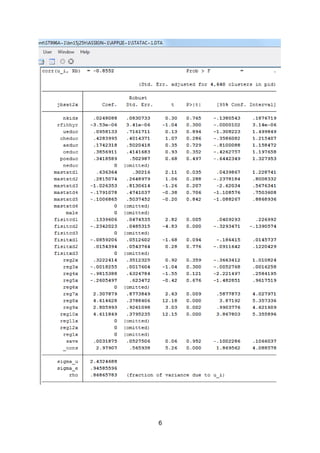
SlideShare a Scribd company logo
1 of 6
1
Leeds University
Business School
Assessed Coursework Coversheet
For use with individual assessed work
Student Identification Number:
Module Code: LUBS5108M01
Module Title: Applied Econometrics
Module Leader: Kausik Chaudhuri
Declared Word Count: 1497
FOR OFFICE USE ONLY
SCRIPT NO.
LATE DAYS
2 0 0 9 9 4 3 6 3
Word count excluding cover page, reference list, and appendices
2
Applied Econometrics: Project 5
Introduction
Using data from the last two waves of the British Household Panel Survey: this project analyses
results from a produced panel data-set consisting of a cross-sectional unit with added regional
dummies. The aim is thus to determine the influence certain factors have on individuals’ job
satisfaction where total pay represents our dependent variable, jbsat2x.
A Random Effects (RE) and Fixed Effects (FE) model were initially performed, holding the
assumption of uncorrelated and correlated individual-specific effects on the independent
variables respectively, with a subsequent Hausman test to compare the previously stored results.
The null hypothesis for such a test is that the Re and Fe are asymptotically equivalent given
exogenous unobserved effects:
𝐻0 ∶ β̂ 𝑅𝐸 = β̂ 𝐹𝐸
Note the standardized coefficient vectors represent the time-varying explanatory variables,
excluding the time variables (McManus, 2011, p.36).
The test results (see Appendix 1) elucidate a significant difference between the results: with a
chi2 of 40.90 and a Prob>chi2 value significant at the 0.05 level (0.0006), thus we reject the null
hypothesis. It can therefore be inferred that the RE model is inconsistent, and hence the FE
model is preferred.
Despite FE being preferred there are some noteworthy drawbacks to the model which need to be
discussed before advancing, as clarified by McManus (2011, p.19); firstly, time-varying
unobserved effects and time-varying measurement error can still exist, and therefore the method
is not a solution for all sources of endogeneity bias. Secondly, as all time-constant effects are
omitted there can be no estimation of effects for gender and race, along with vague estimates
given minor variations in the dataset such as an individual’s education in adulthood. Lastly, the
model ignores between-unit variation and opts to use only within-unit change, whilst allowing for
greater standard errors and an incorrect estimation of the 𝑅2
statistic.
In response to some of these drawbacks; the data used in this project consists of two waves,
(Wave 17 and Wave 18) with many entities, as opposed to numerous waves and limited entities,
thus it can assumed that although not controlling completely of endogeneity bias, time-varying
causes are restricted to a high degree. To attain the correct estimation for the 𝑅2
statistic in the
FE model, an areg function was computed into STATA, resulting in a value of 0.8201 (see
Appendix 2). Thus we can say that 82% of the variance in jbsat2x can be explained by the
independent variables, a relatively high percentage for a model of this type.
Microeconometric datasets used in panels are likely to display cross-sectional correlation and
sequential patterns: thus overlooking, or failing to control for heteroscedasticity could lead to
biased statistical implications. Justifiably the need for a robust estimation of the standard errors
in our FE model is needed, which is attainable in STATA with the command addition of variance-
covariance matrix of estimators - (vce)robust.
The ordering of the explanatory variables in the model allows for control over a base category in
which we can compare the other variable coefficients in that division to. For the purpose of this
project, the controlled variables dropped are: neduc, mastatd6, fisitcd3, fisitxd3, and reg1x, with
the last variable representing London from our regional dummy variables included. Additionally,
male, reg6, reg11x, and reg12x were all omitted due to collinearity.
3
Analysis:
For relevant analysis purposes, only variables which have a significant influence on the
dependent variable will be considered, or more precisely, the variables in which we reject the null
hypothesis (𝐻0) that the coefficient is significantly different from 0 for the corresponding p-value
lower than 0.05. The correlation between errors u_i and the regressors in the fixed effects model
is given as -0.8552 or -85.52% (see Appendix 3 for full data page).
With or without the vce(robust) option, the estimated coefficients remained the same, however a
difference occurred with larger standard errors across the model and slightly differing p-values,
although the difference was minimal enough for the significant variables to remain significant in
both approaches. The F-test is also effected in the cluster robust model, whereby the value is
unreported due to the problematic nature in computing the statistic, it could be that the number of
clusters are too small to support the number of predictors in the model, or perhaps that one or
more of the clusters for one of the variables has no variation.
Despite running the model various times with a different base variable in regards to the
educational category, we fail to reject the 𝐻0 due to large corresponding p-values in each case.
This indicates that the estimations are of little significance to us at the 0.05 or even 0.1 level,
The rho value, or intraclass correlation, of 0.8686 is automatically calculated via the following
formula:
(𝑠𝑖𝑔𝑚𝑎_𝑢)2
(𝑠𝑖𝑔𝑚𝑎_𝑢)2 + (𝑠𝑖𝑔𝑚𝑎_𝑒)2
Where rho represents the correlation of the observations in a cluster, we can infer that 86.9% of
the variance is due to differences across panels. This is an extremely high percentage, and
therefore the less unique any additional information is for each individual in the cluster.
Mastatd1: p-value = 0.035 < 0.05
With a coefficient value of 0.63636, we can infer that a married individual is 63.6% more likely to
be satisfied with his or hers total pay compared to an individual who never married, with regards
to the other six variable categories. The rationale behind such a percentage could be due to the
income from the individuals’ partner whereby they’re jointly comfortable with their finances,
however this insinuates correlation with an unobserved absent variable. Thus the more logical
reasoning behind the percentage value could be due to personal satisfaction with their partner as
opposed to material possessions for an unmarried person. Note: these assumptions are clearly
speculative and do not represent any empirical findings.
Fisitcd1: p-value = 0.005 < 0.05
In regards to a change in an individual’s financial situation compared to the previous year, with a
coefficient value of 0.13396 we can infer that an individual who is financially better off is 13.4%
more likely to be satisfied with their total pay compared to an individual whose financial situation
is about the same as the previous year, with regards to the other six variable categories.
Although it would be easy to hypothesise this percentage to be extremely high, the variable is
unable to elaborate the measureable extent in which an individual’s financial situation is better
off, and therefore it could be any additional amount. Furthermore the source of an increase in
finances is unstipulated and could be unrelated to an individuals’ total pay from employment,
hence the relatively low percentage in regards to satisfaction for total pay.
4
Fisitcd2: p-value = 0.000 < 0.05
Similarly as before, in regards to a change in an individual’s financial situation compared to the
previous year, with a coefficient value of -0.23420 we can infer that an individual is 23.4% less
likely to be satisfied with their total pay when they’re worse off compared to an individual who is
about the same in the previous year, with regards to the other six variable categories. The
absolute coefficient from this variable was expected to be higher than fisitcd1 as being financially
worse off than the previous year would directly cause a decrease in satisfaction regardless of the
circumstances for the individual, and hence more liability would be directed at an individuals’ total
pay value.
Reg7x: p-value = 0.009 < 0.05
With a coefficient value of 2.30788, we can infer that an individual residing in the North-West of
the UK is 2.3 times more likely to be satisfied with their total pay compared to an individual who
lives in London, with regards to the other six variable categories.
Reg8x: p-value = 0.000 < 0.05
With a coefficient value of 4.61463, we can infer that an individual living in Yorkshire and the
Humber is 4.6 times more likely to be satisfied with their total pay compared to an individual who
lives in London, with regards to the other six variable categories.
Reg9x: p-value = 0.002 < 0.05
With a coefficient value of 2.80599, we can infer that an individual who lives in the North-East of
the UK is 2.8 times more likely to be satisfied with their total pay compared to an individual who
lives in London, with regards to the other six variable categories.
Reg10x: p-value = 0.000 < 0.05
With a coefficient value of 4.61185, we can infer that an individual situated in Wales is 4.6 times
more likely to be satisfied with their total pay compared to an individual who lives in London, with
regards to the other six variable categories.
Collectively reporting on the significant regional dummies is simplified due to the results, whereby
individuals residing outside of London are at least more than two times likely to be satisfied with
their total pay as opposed to living in the capital. The foremost rational behind such a result can
be postulated towards the living costs which are at their highest when living in the capital of
England, and cheaper as you move further north of the country.
5
Reference List
McManus, P.A. 2011. Introduction to Regression Models for Panel Data Analysis. [Online].
[Accessed 14th May 2016]. Available from:
http://www.indiana.edu/~wim/docs/10_7_2011_slides.pdf.
Appendices
Appendix 1:
Appendix 2:
Appendix 3: (on next page for easier viewing)
6

More Related Content

Viewers also liked

The matrix marketting
The matrix markettingThe matrix marketting
The matrix markettingshaniajay
 
Multi-thérapies
Multi-thérapiesMulti-thérapies
Multi-thérapiesITPCMENA
 
الإيدز و الصحة و آلناس لبنان ـ 2005
الإيدز و الصحة و آلناس لبنان ـ 2005الإيدز و الصحة و آلناس لبنان ـ 2005
الإيدز و الصحة و آلناس لبنان ـ 2005ITPCMENA
 
Our own theory of music videos
Our own theory of music videosOur own theory of music videos
Our own theory of music videosksinghmedia
 
Representattion of race
Representattion of raceRepresentattion of race
Representattion of raceshaniajay
 
Operação em supermercados
Operação em supermercadosOperação em supermercados
Operação em supermercadosBruno Crescente
 
ANTIVIRUS
ANTIVIRUSANTIVIRUS
ANTIVIRUSfauscha
 
Magazine layout fp full
Magazine layout fp fullMagazine layout fp full
Magazine layout fp fullBartoszMogilan
 
Xinyi_Gong_podium
Xinyi_Gong_podiumXinyi_Gong_podium
Xinyi_Gong_podiumXinyi Gong
 

Viewers also liked (9)

The matrix marketting
The matrix markettingThe matrix marketting
The matrix marketting
 
Multi-thérapies
Multi-thérapiesMulti-thérapies
Multi-thérapies
 
الإيدز و الصحة و آلناس لبنان ـ 2005
الإيدز و الصحة و آلناس لبنان ـ 2005الإيدز و الصحة و آلناس لبنان ـ 2005
الإيدز و الصحة و آلناس لبنان ـ 2005
 
Our own theory of music videos
Our own theory of music videosOur own theory of music videos
Our own theory of music videos
 
Representattion of race
Representattion of raceRepresentattion of race
Representattion of race
 
Operação em supermercados
Operação em supermercadosOperação em supermercados
Operação em supermercados
 
ANTIVIRUS
ANTIVIRUSANTIVIRUS
ANTIVIRUS
 
Magazine layout fp full
Magazine layout fp fullMagazine layout fp full
Magazine layout fp full
 
Xinyi_Gong_podium
Xinyi_Gong_podiumXinyi_Gong_podium
Xinyi_Gong_podium
 

Similar to 200994363

Logistic regression and analysis using statistical information
Logistic regression and analysis using statistical informationLogistic regression and analysis using statistical information
Logistic regression and analysis using statistical informationAsadJaved304231
 
X18125514 ca2-statisticsfor dataanalytics
X18125514 ca2-statisticsfor dataanalyticsX18125514 ca2-statisticsfor dataanalytics
X18125514 ca2-statisticsfor dataanalyticsShantanu Deshpande
 
Guide for building GLMS
Guide for building GLMSGuide for building GLMS
Guide for building GLMSAli T. Lotia
 
Advanced microeconometric project
Advanced microeconometric projectAdvanced microeconometric project
Advanced microeconometric projectLaurentCyrus
 
Introduction to Econometrics for under gruadute class.pptx
Introduction to Econometrics for under gruadute class.pptxIntroduction to Econometrics for under gruadute class.pptx
Introduction to Econometrics for under gruadute class.pptxtadegebreyesus
 
Applications of regression analysis - Measurement of validity of relationship
Applications of regression analysis - Measurement of validity of relationshipApplications of regression analysis - Measurement of validity of relationship
Applications of regression analysis - Measurement of validity of relationshipRithish Kumar
 
Assigning Scores For Ordered Categorical Responses
Assigning Scores For Ordered Categorical ResponsesAssigning Scores For Ordered Categorical Responses
Assigning Scores For Ordered Categorical ResponsesMary Montoya
 
ECON104RoughDraft1
ECON104RoughDraft1ECON104RoughDraft1
ECON104RoughDraft1John Nguyen
 
GAP Statistical Analysis Report
GAP Statistical Analysis ReportGAP Statistical Analysis Report
GAP Statistical Analysis ReportAlexandra Nolan
 
ders 8 Quantile-Regression.ppt
ders 8 Quantile-Regression.pptders 8 Quantile-Regression.ppt
ders 8 Quantile-Regression.pptErgin Akalpler
 
Biometry regression
Biometry regressionBiometry regression
Biometry regressionmusadoto
 
Econometrics project
Econometrics projectEconometrics project
Econometrics projectShubham Joon
 
Quantifying the Uncertainty of Long-Term Economic Projections
Quantifying the Uncertainty of Long-Term Economic ProjectionsQuantifying the Uncertainty of Long-Term Economic Projections
Quantifying the Uncertainty of Long-Term Economic ProjectionsCongressional Budget Office
 
Project -- Second DeliverableIntroductionAfter reviewing the.docx
Project -- Second DeliverableIntroductionAfter reviewing the.docxProject -- Second DeliverableIntroductionAfter reviewing the.docx
Project -- Second DeliverableIntroductionAfter reviewing the.docxbriancrawford30935
 
Correlation analysis
Correlation analysisCorrelation analysis
Correlation analysisAwais Salman
 
Degree exam 2019 q &amp; a (1) (1)
Degree exam 2019 q &amp; a (1) (1)Degree exam 2019 q &amp; a (1) (1)
Degree exam 2019 q &amp; a (1) (1)OsamaKhan404075
 
Classification via Logistic Regression
Classification via Logistic RegressionClassification via Logistic Regression
Classification via Logistic RegressionTaweh Beysolow II
 
Add slides
Add slidesAdd slides
Add slidesRupa D
 

Similar to 200994363 (20)

Logistic regression and analysis using statistical information
Logistic regression and analysis using statistical informationLogistic regression and analysis using statistical information
Logistic regression and analysis using statistical information
 
X18125514 ca2-statisticsfor dataanalytics
X18125514 ca2-statisticsfor dataanalyticsX18125514 ca2-statisticsfor dataanalytics
X18125514 ca2-statisticsfor dataanalytics
 
Guide for building GLMS
Guide for building GLMSGuide for building GLMS
Guide for building GLMS
 
Advanced microeconometric project
Advanced microeconometric projectAdvanced microeconometric project
Advanced microeconometric project
 
Introduction to Econometrics for under gruadute class.pptx
Introduction to Econometrics for under gruadute class.pptxIntroduction to Econometrics for under gruadute class.pptx
Introduction to Econometrics for under gruadute class.pptx
 
Applications of regression analysis - Measurement of validity of relationship
Applications of regression analysis - Measurement of validity of relationshipApplications of regression analysis - Measurement of validity of relationship
Applications of regression analysis - Measurement of validity of relationship
 
Assigning Scores For Ordered Categorical Responses
Assigning Scores For Ordered Categorical ResponsesAssigning Scores For Ordered Categorical Responses
Assigning Scores For Ordered Categorical Responses
 
ECON104RoughDraft1
ECON104RoughDraft1ECON104RoughDraft1
ECON104RoughDraft1
 
GAP Statistical Analysis Report
GAP Statistical Analysis ReportGAP Statistical Analysis Report
GAP Statistical Analysis Report
 
ders 8 Quantile-Regression.ppt
ders 8 Quantile-Regression.pptders 8 Quantile-Regression.ppt
ders 8 Quantile-Regression.ppt
 
Biometry regression
Biometry regressionBiometry regression
Biometry regression
 
Econometrics project
Econometrics projectEconometrics project
Econometrics project
 
Quantifying the Uncertainty of Long-Term Economic Projections
Quantifying the Uncertainty of Long-Term Economic ProjectionsQuantifying the Uncertainty of Long-Term Economic Projections
Quantifying the Uncertainty of Long-Term Economic Projections
 
Project -- Second DeliverableIntroductionAfter reviewing the.docx
Project -- Second DeliverableIntroductionAfter reviewing the.docxProject -- Second DeliverableIntroductionAfter reviewing the.docx
Project -- Second DeliverableIntroductionAfter reviewing the.docx
 
Multiple regression
Multiple regressionMultiple regression
Multiple regression
 
Correlation analysis
Correlation analysisCorrelation analysis
Correlation analysis
 
Degree exam 2019 q &amp; a (1) (1)
Degree exam 2019 q &amp; a (1) (1)Degree exam 2019 q &amp; a (1) (1)
Degree exam 2019 q &amp; a (1) (1)
 
Classification via Logistic Regression
Classification via Logistic RegressionClassification via Logistic Regression
Classification via Logistic Regression
 
Logistic regression sage
Logistic regression sageLogistic regression sage
Logistic regression sage
 
Add slides
Add slidesAdd slides
Add slides
 

200994363

  • 1. 1 Leeds University Business School Assessed Coursework Coversheet For use with individual assessed work Student Identification Number: Module Code: LUBS5108M01 Module Title: Applied Econometrics Module Leader: Kausik Chaudhuri Declared Word Count: 1497 FOR OFFICE USE ONLY SCRIPT NO. LATE DAYS 2 0 0 9 9 4 3 6 3 Word count excluding cover page, reference list, and appendices
  • 2. 2 Applied Econometrics: Project 5 Introduction Using data from the last two waves of the British Household Panel Survey: this project analyses results from a produced panel data-set consisting of a cross-sectional unit with added regional dummies. The aim is thus to determine the influence certain factors have on individuals’ job satisfaction where total pay represents our dependent variable, jbsat2x. A Random Effects (RE) and Fixed Effects (FE) model were initially performed, holding the assumption of uncorrelated and correlated individual-specific effects on the independent variables respectively, with a subsequent Hausman test to compare the previously stored results. The null hypothesis for such a test is that the Re and Fe are asymptotically equivalent given exogenous unobserved effects: 𝐻0 ∶ β̂ 𝑅𝐸 = β̂ 𝐹𝐸 Note the standardized coefficient vectors represent the time-varying explanatory variables, excluding the time variables (McManus, 2011, p.36). The test results (see Appendix 1) elucidate a significant difference between the results: with a chi2 of 40.90 and a Prob>chi2 value significant at the 0.05 level (0.0006), thus we reject the null hypothesis. It can therefore be inferred that the RE model is inconsistent, and hence the FE model is preferred. Despite FE being preferred there are some noteworthy drawbacks to the model which need to be discussed before advancing, as clarified by McManus (2011, p.19); firstly, time-varying unobserved effects and time-varying measurement error can still exist, and therefore the method is not a solution for all sources of endogeneity bias. Secondly, as all time-constant effects are omitted there can be no estimation of effects for gender and race, along with vague estimates given minor variations in the dataset such as an individual’s education in adulthood. Lastly, the model ignores between-unit variation and opts to use only within-unit change, whilst allowing for greater standard errors and an incorrect estimation of the 𝑅2 statistic. In response to some of these drawbacks; the data used in this project consists of two waves, (Wave 17 and Wave 18) with many entities, as opposed to numerous waves and limited entities, thus it can assumed that although not controlling completely of endogeneity bias, time-varying causes are restricted to a high degree. To attain the correct estimation for the 𝑅2 statistic in the FE model, an areg function was computed into STATA, resulting in a value of 0.8201 (see Appendix 2). Thus we can say that 82% of the variance in jbsat2x can be explained by the independent variables, a relatively high percentage for a model of this type. Microeconometric datasets used in panels are likely to display cross-sectional correlation and sequential patterns: thus overlooking, or failing to control for heteroscedasticity could lead to biased statistical implications. Justifiably the need for a robust estimation of the standard errors in our FE model is needed, which is attainable in STATA with the command addition of variance- covariance matrix of estimators - (vce)robust. The ordering of the explanatory variables in the model allows for control over a base category in which we can compare the other variable coefficients in that division to. For the purpose of this project, the controlled variables dropped are: neduc, mastatd6, fisitcd3, fisitxd3, and reg1x, with the last variable representing London from our regional dummy variables included. Additionally, male, reg6, reg11x, and reg12x were all omitted due to collinearity.
  • 3. 3 Analysis: For relevant analysis purposes, only variables which have a significant influence on the dependent variable will be considered, or more precisely, the variables in which we reject the null hypothesis (𝐻0) that the coefficient is significantly different from 0 for the corresponding p-value lower than 0.05. The correlation between errors u_i and the regressors in the fixed effects model is given as -0.8552 or -85.52% (see Appendix 3 for full data page). With or without the vce(robust) option, the estimated coefficients remained the same, however a difference occurred with larger standard errors across the model and slightly differing p-values, although the difference was minimal enough for the significant variables to remain significant in both approaches. The F-test is also effected in the cluster robust model, whereby the value is unreported due to the problematic nature in computing the statistic, it could be that the number of clusters are too small to support the number of predictors in the model, or perhaps that one or more of the clusters for one of the variables has no variation. Despite running the model various times with a different base variable in regards to the educational category, we fail to reject the 𝐻0 due to large corresponding p-values in each case. This indicates that the estimations are of little significance to us at the 0.05 or even 0.1 level, The rho value, or intraclass correlation, of 0.8686 is automatically calculated via the following formula: (𝑠𝑖𝑔𝑚𝑎_𝑢)2 (𝑠𝑖𝑔𝑚𝑎_𝑢)2 + (𝑠𝑖𝑔𝑚𝑎_𝑒)2 Where rho represents the correlation of the observations in a cluster, we can infer that 86.9% of the variance is due to differences across panels. This is an extremely high percentage, and therefore the less unique any additional information is for each individual in the cluster. Mastatd1: p-value = 0.035 < 0.05 With a coefficient value of 0.63636, we can infer that a married individual is 63.6% more likely to be satisfied with his or hers total pay compared to an individual who never married, with regards to the other six variable categories. The rationale behind such a percentage could be due to the income from the individuals’ partner whereby they’re jointly comfortable with their finances, however this insinuates correlation with an unobserved absent variable. Thus the more logical reasoning behind the percentage value could be due to personal satisfaction with their partner as opposed to material possessions for an unmarried person. Note: these assumptions are clearly speculative and do not represent any empirical findings. Fisitcd1: p-value = 0.005 < 0.05 In regards to a change in an individual’s financial situation compared to the previous year, with a coefficient value of 0.13396 we can infer that an individual who is financially better off is 13.4% more likely to be satisfied with their total pay compared to an individual whose financial situation is about the same as the previous year, with regards to the other six variable categories. Although it would be easy to hypothesise this percentage to be extremely high, the variable is unable to elaborate the measureable extent in which an individual’s financial situation is better off, and therefore it could be any additional amount. Furthermore the source of an increase in finances is unstipulated and could be unrelated to an individuals’ total pay from employment, hence the relatively low percentage in regards to satisfaction for total pay.
  • 4. 4 Fisitcd2: p-value = 0.000 < 0.05 Similarly as before, in regards to a change in an individual’s financial situation compared to the previous year, with a coefficient value of -0.23420 we can infer that an individual is 23.4% less likely to be satisfied with their total pay when they’re worse off compared to an individual who is about the same in the previous year, with regards to the other six variable categories. The absolute coefficient from this variable was expected to be higher than fisitcd1 as being financially worse off than the previous year would directly cause a decrease in satisfaction regardless of the circumstances for the individual, and hence more liability would be directed at an individuals’ total pay value. Reg7x: p-value = 0.009 < 0.05 With a coefficient value of 2.30788, we can infer that an individual residing in the North-West of the UK is 2.3 times more likely to be satisfied with their total pay compared to an individual who lives in London, with regards to the other six variable categories. Reg8x: p-value = 0.000 < 0.05 With a coefficient value of 4.61463, we can infer that an individual living in Yorkshire and the Humber is 4.6 times more likely to be satisfied with their total pay compared to an individual who lives in London, with regards to the other six variable categories. Reg9x: p-value = 0.002 < 0.05 With a coefficient value of 2.80599, we can infer that an individual who lives in the North-East of the UK is 2.8 times more likely to be satisfied with their total pay compared to an individual who lives in London, with regards to the other six variable categories. Reg10x: p-value = 0.000 < 0.05 With a coefficient value of 4.61185, we can infer that an individual situated in Wales is 4.6 times more likely to be satisfied with their total pay compared to an individual who lives in London, with regards to the other six variable categories. Collectively reporting on the significant regional dummies is simplified due to the results, whereby individuals residing outside of London are at least more than two times likely to be satisfied with their total pay as opposed to living in the capital. The foremost rational behind such a result can be postulated towards the living costs which are at their highest when living in the capital of England, and cheaper as you move further north of the country.
  • 5. 5 Reference List McManus, P.A. 2011. Introduction to Regression Models for Panel Data Analysis. [Online]. [Accessed 14th May 2016]. Available from: http://www.indiana.edu/~wim/docs/10_7_2011_slides.pdf. Appendices Appendix 1: Appendix 2: Appendix 3: (on next page for easier viewing)
  • 6. 6