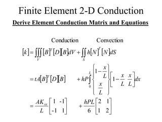
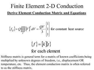
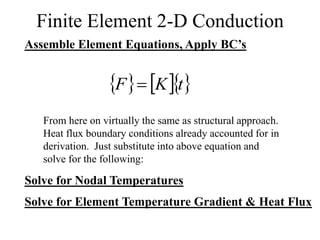
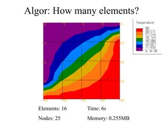
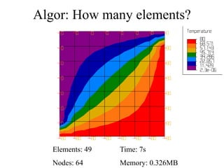
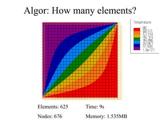
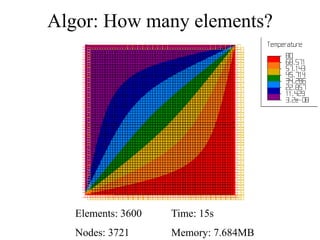
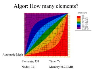
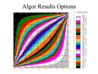
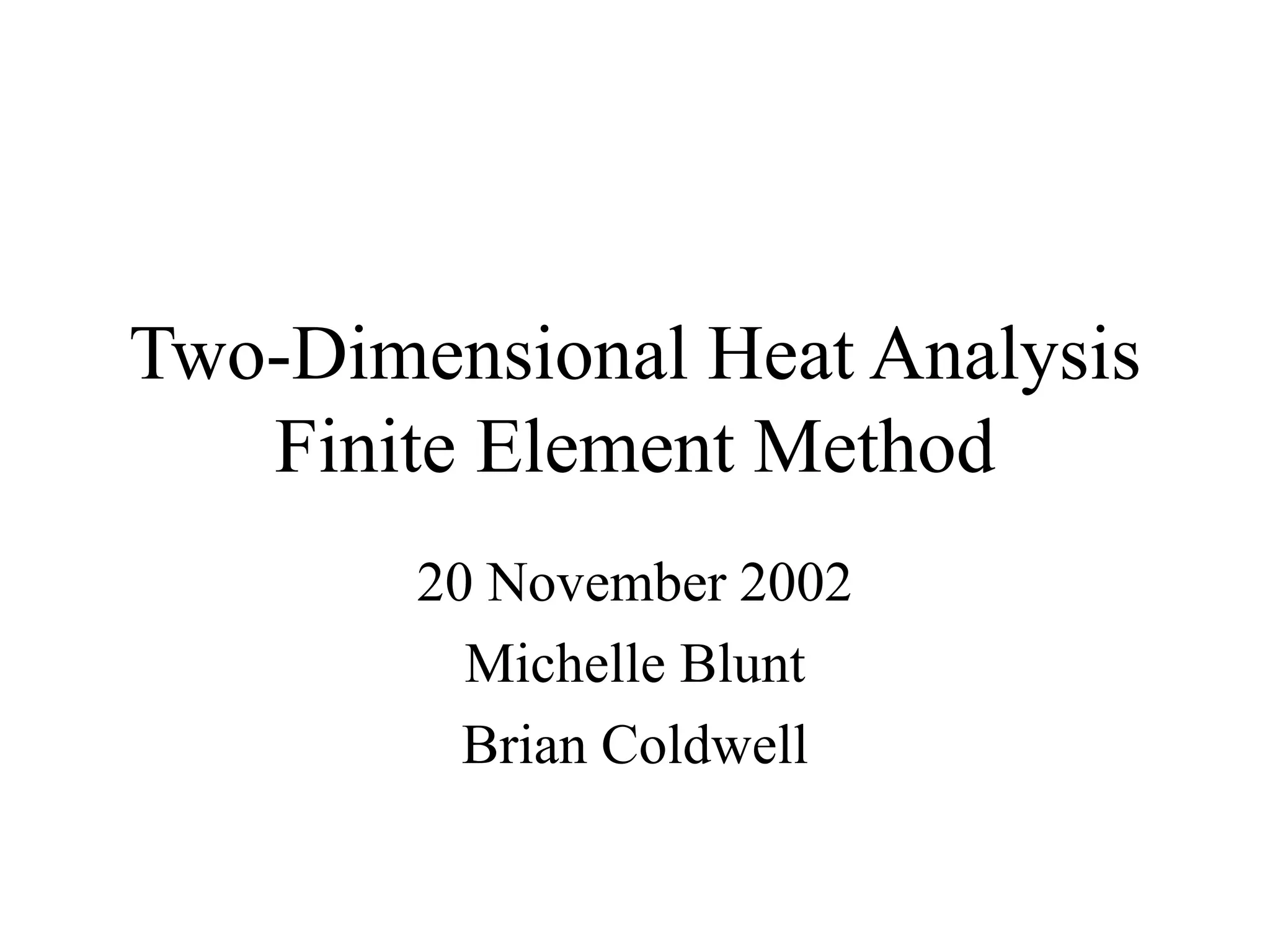
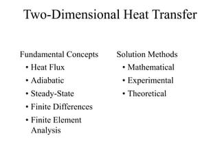
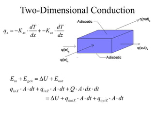
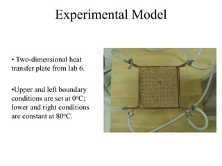
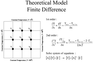
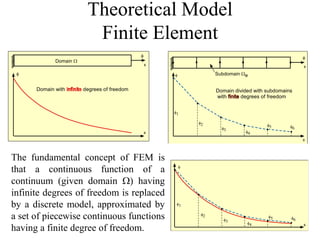
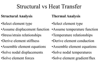
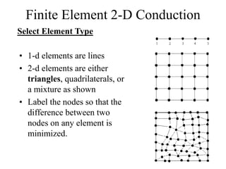
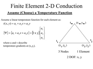
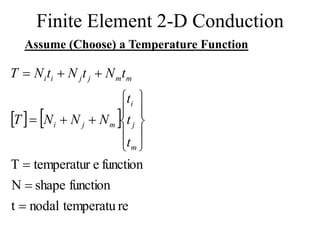
This document discusses two-dimensional heat transfer analysis using the finite element method. It begins with an overview of fundamental heat transfer concepts and solution methods such as steady-state, finite differences, and finite elements. It then describes the theoretical finite element model, including assuming a temperature function over elements, defining temperature gradient relationships, deriving the element conduction matrix, and assembling element equations. The document also discusses applying boundary conditions and solving for nodal temperatures and heat fluxes. It provides examples of applying the method to different numbers of elements. In the end, it discusses tradeoffs between mesh size and computational resources.
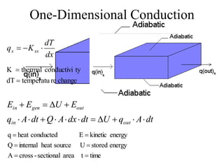
![Finite Element 2-D Conduction
Define Temperature Gradient Relationships
m
j
i
m
j
i
m
j
i
m
j
i
m
j
i
x
N
x
B
t
t
t
y
N
y
N
y
N
x
N
x
N
x
N
y
T
x
T
g
1
Analogous to strain
matrix: {g}=[B]{t}
[B] is derivative of [N]
g
D
g
q
q
y
x
yy
xx
K
0
0
K
:
Gradient
rature
flux/Tempe
Heat](https://image.slidesharecdn.com/heat-240131105544-b1158266/85/Heat-analysis-finite-element-method-two-Dimensional-12-320.jpg)