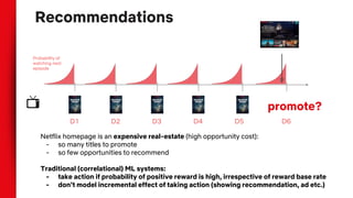
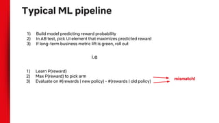
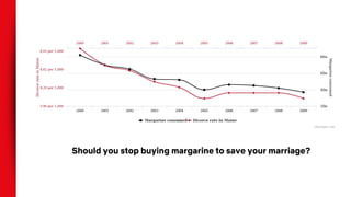
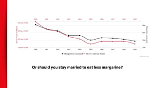
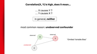
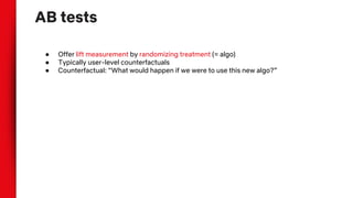
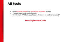
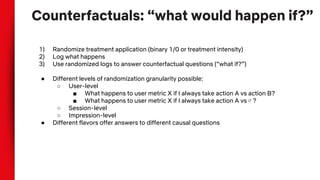
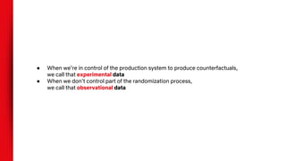
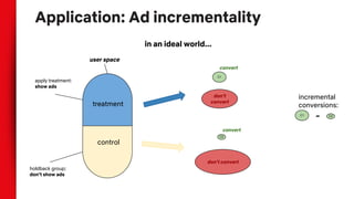
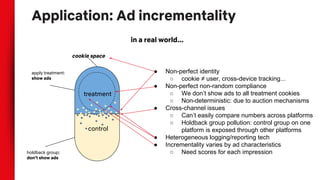
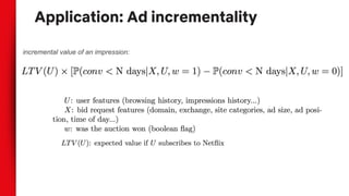
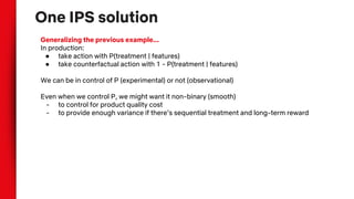
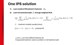
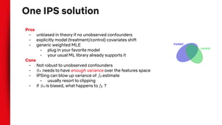
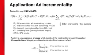
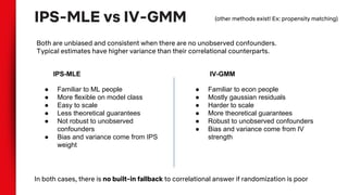
This document discusses causal inference techniques for machine learning, including: - Correlation does not imply causation, and observational data can be biased by confounding variables. Randomization and counterfactual modeling are introduced as alternatives. - Inverse propensity scoring is presented as a method for estimating treatment effects from observational data by reweighting samples based on their propensity to receive treatment. 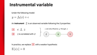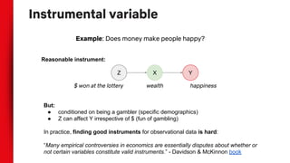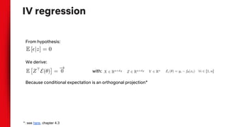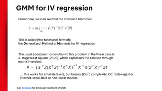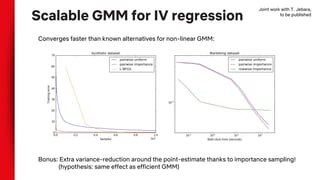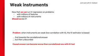- Instrumental variable regression is discussed as another technique, using variables that influence the treatment but not the outcome except through treatment. Scalable methods for instrumental variable regression on large datasets are proposed. 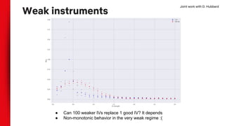- Challenges with weak instruments are noted, as instrumental variable estimates can become more biased than purely correlational models when instruments are weak

1. Benoît Rostykus
Senior Machine Learning Researcher
without headaches
March 2018

2. ● Correlation ≠ causation
● Randomization & counterfactuals
● Experimental vs observational data
● Inverse Propensity Scoring
● Instrumental variables
○ Generalized Method of Moments
○ Scalable IV regression
○ Weak instruments
● Conclusion
Content

3. Correlation ≠ causation

4. Should you stop buying margarine to save your marriage?

5. Or should you stay married to eat less margarine?

6. Correlation(X, Y) is high, does it mean...
… X causes Y ?
… Y causes X ?
in general, neither
X
Y
C
most common reason: unobserved confounder
observed
observed
unobserved
“Omitted Variable Bias”

7. W1 W2 W3 W4 W5
advertise?
Probability of
buying diapers
tomorrow
Advertising
W6
● High probability of conversion the day before weekly groceries irrespective of adverts shown
● Effect of Pampers ads is null in this case.
Traditional (correlational) machine learning will fail and waste $ on useless ads
in practice, Cost-Per-Incremental-Acquisition can be > 100x Cost-Per-Acquisition (!!!!!)

8. D1 D2 D3 D4 D5
promote?
Probability of
watching next
episode
Recommendations
D6
Netflix homepage is an expensive real-estate (high opportunity cost):
- so many titles to promote
- so few opportunities to recommend
Traditional (correlational) ML systems:
- take action if probability of positive reward is high, irrespective of reward base rate
- don’t model incremental effect of taking action (showing recommendation, ad etc.)

9. Surely we can do better.

10. Randomization &
counterfactuals

11. Typical ML pipeline
1) Build model predicting reward probability
2) In AB test, pick UI element that maximizes predicted reward
3) If long-term business metric lift is green, roll out

12. Typical ML pipeline
1) Build model predicting reward probability
2) In AB test, pick UI element that maximizes predicted reward
3) If long-term business metric lift is green, roll out
1) Learn P(reward)
2) Max P(reward) to pick arm
3) Evaluate on #(rewards | new policy) - #(rewards | old policy)
i.e

13. Typical ML pipeline
1) Build model predicting reward probability
2) In AB test, pick UI element that maximizes predicted reward
3) If long-term business metric lift is green, roll out
1) Learn P(reward)
2) Max P(reward) to pick arm
3) Evaluate on #(rewards | new policy) - #(rewards | old policy)
i.e
mismatch!

14. AB tests
● Offer lift measurement by randomizing treatment (= algo)
● Typically user-level counterfactuals
● Counterfactual: “What would happen if we were to use this new algo?”

15. AB tests
● Offer lift measurement by randomizing treatment (= algo)
● Typically user-level counterfactuals
● Counterfactual: “What would happen if we were to use this new algo?”
We can generalize this!

16. Counterfactuals: “what would happen if?”
1) Randomize treatment application (binary 1/0 or treatment intensity)
2) Log what happens
3) Use randomized logs to answer counterfactual questions (“what if?”)
● Different levels of randomization granularity possible:
○ User-level
■ What happens to user metric X if I always take action A vs action B?
■ What happens to user metric X if I always take action A vs ∅ ?
○ Session-level
○ Impression-level
● Different flavors offer answers to different causal questions

17. Experimental vs
observational data

18. ● When we’re in control of the production system to produce counterfactuals,
we call that experimental data
● When we don’t control part of the randomization process,
we call that observational data

19. Incrementality modeling
Simple experimental example
● On X% of traffic, take no action (or random action)
● On (100-X)% of traffic, take action
● X is typically small because it has a product cost (quality / efficiency / …)
● From collected data, learn:
○ P(reward | features, action) = f(features)
○ P(reward | features, no action) = g(features)
○ Predicted lift: lift(features) = f(features) - g(features)
● Use incremental model in production:
○ Max over arms of lift(features(arm))

20. Incrementality modeling
Pros
● simple
● no model assumptions, plug your favorite ML technique
Cons
● 2 models
● X is small
○ limit on g model accuracy
○ asymmetrical
● doesn’t explicitly model lift
○ can be hard to calibrate
○ offline metrics?

21. Inverse Propensity Scoring

22. One IPS solution
Generalizing the previous example...
In production:
● take action with P(treatment | features)
● take counterfactual action with 1 - P(treatment | features)
We can be in control of P (experimental) or not (observational)
Even when we control P, we might want it non-binary (smooth)
- to control for product quality cost
- to provide enough variance if there’s sequential treatment and long-term reward

23. One IPS solution
1) Learn model of P(treatment | features)
2) Learn incremental model through weighted MLE:
: treatment variable (usually binary)
: predicted lift
and can have different features set
if sequential treatment, need to condition on full treatment path

24. One IPS solution
Pros
- unbiased in theory if no unobserved confounders
- explicitly model (treatment/control) covariates shift
- generic weighted MLE
- plug in your favorite model
- your usual ML library already supports it
Cons
- Not robust to unobserved confounders
- needs to have enough variance over the features space
- IPSing can blow up variance of estimate
- usually resort to clipping
- if is biased, what happens to ?
treated
control

25. Application: Ad incrementality
Does online advertising work?

26. Application: Ad incrementality
article, 02/08/2018
clickbait headlines:
article, 07/27/2017

27. Application: Ad incrementality
Main problem: measurement
Advertising platforms report on metrics such as Cost-Per-Click (CPC) or
Cost-Per-Action (CPA)
Based on attribution methodologies such as:
- Last click (only give credit to the last ad clicked before conversion)
- Last view (only give credit to the last ad viewed)
- Any view (any ad “viewed” gets the credit)
- Arbitrary combinations of the previous with fudge factors
...These are non-rigorous ways of estimating causal effect of an ad
In practice metrics reported over-inflate ad effect by 1 or 2 orders of magnitude
… because most people would convert anyway, irrespective of the ad
Cost-Per-Incremental-Action > 100x CPA
Rigorous alternative:
1) proper lift measurement using counterfactuals (“ghost bids” / “ghost ads”)
2) Incrementality-based bidding to optimize for ad effect

28. Application: Ad incrementality
in an ideal world...
don’t
convert
don’t convert
C1
C2
C1 C2
-
incremental
conversions:
holdback group:
don’t show ads
apply treatment:
show ads
control
treatment
user space
convert
convert

29. Application: Ad incrementality
in a real world...
control
treatment
cookie space
● Non-perfect identity
○ cookie ≠ user, cross-device tracking...
● Non-perfect non-random compliance
○ We don’t show ads to all treatment cookies
○ Non-deterministic: due to auction mechanisms
● Cross-channel issues
○ Can’t easily compare numbers across platforms
○ Holdback group pollution: control group on one
platform is exposed through other platforms
● Heterogeneous logging/reporting tech
● Incrementality varies by ad characteristics
○ Need scores for each impression
apply treatment:
show ads
holdback group:
don’t show ads

30. Application: Ad incrementality
incremental value of an impression:

31. Application: Ad incrementality
Trained through MLE with IPS:
bids = impressions + lost auctions
}
Auction is a non-random process which decides if the treatment (impression) is applied
We need to learn it to get an unbiased estimate of the treatment effect:

32. Instrumental variables

33. Instrumental variable
Under the following model:
An instrument is an observed variable following the 2 properties:
is correlated with
1
2 X YZ
can only influence through
1In practice, we replace with a weaker hypothesis:

34. Instrumental variable
Example: Does money make people happy?
X YZ
$ won at the lottery happinesswealth
Reasonable instrument:
But:
● conditioned on being a gambler (specific demographics)
● Z can affect Y irrespective of $ (fun of gambling)
In practice, finding good instruments for observational data is hard:
“Many empirical controversies in economics are essentially disputes about whether or
not certain variables constitute valid instruments.” - Davidson & McKinnon book

35. Instrumental variable (IV) Regression
● The idea is that we can debias our model by using the
fact that our instruments explain the endogenous
features independently from the regression residual
● Bread and butter of econometrics
○ Because we don’t have parallel universes to run
AB tests on economic policies
○ Observational data is sometimes all we have
Let’s dive into the details since it is less familiar to people with an ML background

36. IV regression
From hypothesis:
We derive:
with:
*: see here, chapter 4.3
Because conditional expectation is an orthogonal projection*

37. GMM for IV regression
From there, we can see that the inference becomes:
See this book for thorough treatment of GMM
This is called (the functional form of):
the Generalized Method of Moments for IV regression
The usual econometrics solution to this problem in the linear case is
2-stage least square (2SLS), which expresses the solution through
matrix inversion:
… this works for small datasets, but breaks (O(n3
) complexity, O(n2
) storage) for
internet-scale data or non-linear models

38. Scalable GMM for IV regression
We are trying to minimize:
Joint work with T. Jebara,
to be published
We want a solution that scales linearly with:
- # of training points
- # of non-zero features per row (sparse high dimensional X)
- # of non-zero instruments per row (sparse high dimensional Z)
or:

39. Scalable GMM for IV regression
More likely to sample rows which matter (large instruments): will converge fast
Idea: pairwise importance-sampling SGD
Joint work with T. Jebara,
to be published

40. Scalable GMM for IV regression
Bonus: Extra variance-reduction around the point-estimate thanks to importance sampling!
(hypothesis: same effect as efficient GMM)
Converges faster than known alternatives for non-linear GMM:
Joint work with T. Jebara,
to be published

41. Weak instruments
Now that we can run IV regression on problems:
- with millions of features
- with millions of instruments
Should we do it?
Problem: when instruments are weak (low correlation with X), the IV estimator is biased
… first towards the correlational answer
… but then unbounded
Causal answer can become worse than correlational one with IV too!
Joint work with D. Hubbard

42. Weak instruments
Simple 1D experiment
observed: hours, z, y
unobserved: wealth
Try to recover:
Joint work with D. Hubbard

43. Weak instruments
● Can 100 weaker IVs replace 1 good IV? It depends
● Non-monotonic behavior in the very weak regime :(
Joint work with D. Hubbard

44. Weak instruments
Controlling for instruments quality is crucial
How to do it in a meaningful and scalable way?
● Partial answer from the statistics literature:
○ Partial F-tests
○ Cragg–Donald
○ Anderson-Rubin
○ …
● “Regularize” the instruments
○ Which cross-validation metric to use? Circular problem. No ground truth!
○ See Hausman Causal Correction from Lewis & Wong
Joint work with D. Hubbard

45. IPS-MLE vs IV-GMM
Both are unbiased and consistent when there are no unobserved confounders.
Typical estimates have higher variance than their correlational counterparts.
IPS-MLE IV-GMM
● Familiar to ML people
● More flexible on model class
● Easy to scale
● Less theoretical guarantees
● Not robust to unobserved
confounders
● Bias and variance come from IPS
weight
● Familiar to econ people
● Mostly gaussian residuals
● Harder to scale
● More theoretical guarantees
● Robust to unobserved confounders
● Bias and variance come from IV
strength
In both cases, there is no built-in fallback to correlational answer if randomization is poor
(other methods exist! Ex: propensity matching)

46. Conclusion

47. Applications
Plenty of use cases for causal inference at Netflix
● Advertising
● Causal recommendations
● Content valuation
● Increased experimentation power
● ...

48. Causal inference in practice
Hard! because:
Causal effects are small
Asymptotic unbiasedness is useless if the variance dominates, even on large datasets
Variance grows even more when there is sequential treatment
Unobserved confounders can have bigger magnitude than what we try to measure
Plenty of unsatisfactory / unanswered questions in the literature
No clean ground-truth
All estimators have their flaws.
Hard (impossible) to measure and compare biases offline on large-scale problems

49. When it matters
Correlational models are fine...
● When we only care about fitting the data / predicting
● When your model predictions won’t interact with the product
Causal models can help...
● When there’s a “why?”
○ “why did NFLX stock price move today?”
● When there’s a “what would happen if?”
○ “what would happen to streaming if iOS app was 10% slower?”
● To build cost-efficient ML algorithms
○ incremental models factor in the effect of taking the action suggested
○ aligned with business metrics lift : maximize likelihood of green AB test
○ … it’s just a greedy one-step-ahead Reinforcement Learning strategy

50. Thank you.