Graphs.pptx

1
UNIVERSITY INSTITUTE OF
COMPUTING
Graphs

GRAPH
• A graph is collection of objects where a set of objects are connected through links.
The connected objects can be represented as vertices, the links which join the
vertices are known as edges.
• Graph can be represented as a pair of sets (V, E), in which V is set of graph
vertices & E is set of joining edges. Consider the following graph
2
Fig 1: Graph [1]

Important Terms In Graph
• Adjacent nodes or neighbors For every edge, e = (u, v) that connects nodes u and v, the nodes u
and v are the end-points and are said to be the adjacent nodes or neighbors.
• Degree of a node Degree of a node u, deg(u), is the total number of edges containing the node u. If
deg(u) = 0, it means that u does not belong to any edge and such a node is known as an isolated
node.
• Regular graph It is a graph where each vertex has the same number of neighbors. That is, every
node has the same degree. A regular graph with vertices of degree k is called a k–regular graph or a
regular graph of degree k. Figure 2 shows regular graphs
3
Fig 2: Regular Graph [2]

Path A path P written as P = {v0, v1, v2, ..., vn), of length n from a node u to v is defined as a
sequence of (n+1) nodes. Here, u = v0, v = vn and vi–1 is adjacent to vi for i = 1, 2, 3,..., n.
Closed path A path P is known as a closed path if the edge has the same end-points. That is, if
v0 = vn.
Simple path A path P is known as a simple path if all the nodes in the path are distinct with an
exception that v0 may be equal to vn. If v0 = vn, then the path is called a closed simple path.
Cycle A path in which the first and the last vertices are same. A simple cycle has no repeated
edges or vertices (except the first and last vertices).
Connected graph A graph is said to be connected if for any two vertices (u, v) in V there is a
path from u to v. That is to say that there are no isolated nodes in a connected graph. A
connected graph that does not have any cycle is called a tree. Therefore, a tree is treated as a
special graph. Figure 3 (a) shows a Tree.
4

Complete graph A graph G is said to be complete if all its nodes are fully connected.
That is, there is a path from one node to every other node in the graph. A complete
graph has n(n–1)/2 edges, where n is the number of nodes in G.
Clique In an undirected graph G = (V, E), clique is a subset of the vertex set C Õ V,
such that for every two vertices in C, there is an edge that connects two vertices.
Labeled graph or weighted graph A graph is said to be labeled if every edge in the
graph is assigned some data. In a weighted graph, the edges of the graph are assigned
some weight or length. The weight of an edge denoted by w(e) is a positive value
which indicates the cost of traversing the edge. Figure 3(c) shows a weighted graph.
Multiple edges Distinct edges which connect the same end-points are called multiple
edges. That is, e = (u, v) and e' = (u, v) are known as multiple edges of G.
5

Loop An edge that has identical end-points is called a loop. That is, e = (u, u).
Multi-graph A graph with multiple edges and/or loops is called a multi-graph. Figure
3 (a) shows a multi-graph.
Size of a graph The size of a graph is the total number of edges in it.
6
Fig 3: Multi-graph, Tree, Weighted Graph [2]

Directed Graph
• If a graph contains ordered pair of vertices, is said to be a Directed Graph.
• If an edge is represented using a pair of vertices (V1, V2), the edge is said to be directed from V1 to V2.
• The first element of the pair V1 is called the start vertex and the second element of the pair V2 is called
the end vertex.
• Set of Vertices V = {1, 2, 3, 4, 5, 5}
• Set of Edges W = {(1, 3), (1, 5), (2, 1), (2, 3), (2, 4), (3, 4), (4, 5)}
7
Fig 4: Directed Graph [3]

Terminology of a Directed Graph
Out-degree of a node The out-degree of a node u, written as outdeg(u), is the
number of edges that originate at u.
In-degree of a node The in-degree of a node u, written as indeg(u), is the number of
edges that terminate at u.
Degree of a node The degree of a node, written as deg(u), is equal to the sum of in-
degree and out-degree of that node. Therefore, deg(u) = indeg(u) + outdeg(u).
Isolated vertex A vertex with degree zero. Such a vertex is not an end-point of any
edge.
Pendant vertex (also known as leaf vertex) A vertex with degree one.
Cut vertex A vertex which when deleted would disconnect the remaining graph.
Source A node u is known as a source if it has a positive out-degree but a zero in-
degree.
Sink A node u is known as a sink if it has a positive in-degree but a zero out-degree.
8

Reachability A node v is said to be reachable from node u, if and only if there exists
a (directed) path from node u to node v. For example, if you consider the directed
graph given in Fig. 5(a), you will observe that node D is reachable from node A.
Strongly connected directed graph A digraph is said to be strongly connected if and
only if there exists a path between every pair of nodes in G. That is, if there is a path
from node u to v, then there must be a path from node v to u.
Unilaterally connected graph A digraph is said to be unilaterally connected if there
exists a path between any pair of nodes u, v in G such that there is a path from u to v
or a path from v to u, but not both.
Weakly connected digraph A directed graph is said to be weakly connected if it is
connected by ignoring the direction of edges. That is, in such a graph, it is possible
to reach any node from any other node by traversing edges in any direction (may not
be in the direction they point). The nodes in a weakly connected directed graph must
have either out-degree or in-degree of at least 1.
9

Parallel/Multiple edges Distinct edges which connect the same end-points are called
multiple edges. That is, e = (u, v) and e' = (u, v) are known as multiple edges of G.
In Fig. 5(a), e3 and e5 are multiple edges connecting nodes C and D.
Simple directed graph A directed graph G is said to be a simple directed graph if
and only if it has no parallel edges. However, a simple directed graph may contain
cycles with an exception that it cannot have more than one loop at a given node.
10
Fig 5: (a) Directed acyclic graph and (b) strongly connected directed acyclic graph [2]

Undirected Graph
• If a graph contains unordered pair of vertices, is said to be an Undirected Graph.
• In this graph, pair of vertices represents the same edge.
• Set of Vertices V = {1, 2, 3, 4, 5}
• Set of Edges E = {(1, 2), (1, 3), (1, 5), (2, 1), (2, 3), (2, 4), (3, 4), (4, 5)}
• In an undirected graph, the nodes are connected by undirected arcs.
• It is an edge that has no arrow. Both the ends of an undirected arc are equivalent, there is
no head or tail.
11
Fig 6: Undirected Graph [3]

Graph Operations
Different operations on graph:
• Add Vertex − Adds a vertex to the graph.
• Add Edge − Adds an edge between the two vertices of the graph.
• Display Vertex − Displays a vertex of the graph.
12

Representation Of Graph
13
There are three common ways of storing graphs in the computer’s memory. They
are:
• Sequential representation by using an adjacency matrix.
• Linked representation by using an adjacency list that stores the neighbors of a
node using a linked list.
• Adjacency multi-list which is an extension of linked representation.

Adjacency Matrix
14
Fig 7: adjacency matrix[4]
Let G=(V,E) be a graph with n vertices. The
adjacency matrix of G is a two-dimensional n by
n array, say adj_mat
If the edge (vi, vj) is in E(G), adj_mat[i][j]=1
If there is no such edge in E(G), adj_mat[i][j]=0
The adjacency matrix for an undirected graph is
symmetric; the adjacency matrix for a digraph
need not be symmetric .

Adjacency Matrix
Graph can be divided into two categories:
a. Sparse graph contains less number of edges.
b. Dense graph contains number of edges as compared to sparse graph.
Adjacency matrix is best for dense graph, but for sparse graph, it is not required.
Adjacency matrix is good solution for dense graph which implies having constant
number of vertices.
Adjacency matrix of an undirected graph is always a symmetric matrix which means
an edge (i, j) implies the edge (j, i).
15

Adjacency Matrix
.
16
The above graph represents undirected graph with the adjacency matrix representation. It shows adjacency
matrix of undirected graph is symmetric. If there is an edge (2, 4), there is also an edge (4, 2).
Fig 8: adjacency matrix[5]

Adjacency Matrix
.
17
Adjacency matrix of a directed graph is never symmetric adj[i][j] = 1, indicated a directed edge from vertex i to
vertex j.
Fig 9: Undirected graph and adjacency matrix[5]

Adjacency Matrix
.
18
The above graph represents directed graph with the adjacency matrix representation. It shows adjacency
matrix of directed graph which is never symmetric. If there is an edge (2, 4), there is not an edge (4, 2). It
indicates direct edge from vertex i to vertex j.
Fig 10: Directed graph and adjacency matrix[5]

Advantages of Adjacency Matrix
• Adjacency matrix representation of graph is very simple to implement.
• Adding or removing time of an edge can be done in O(1) time. Same time is
required to check, if there is an edge between two vertices.
• It is very convenient and simple to program.
19

Disadvantages of Adjacency Matrix
• It consumes huge amount of memory for storing big graphs.
• It requires huge efforts for adding or removing a vertex. If you are constructing a
graph in dynamic structure, adjacency matrix is quite slow for big graphs.
20

Adjacency List
• Adjacency list is another representation of graphs.
• It is a collection of unordered list, used to represent a finite graphs.
• Each list describes the set of neighbors of a vertex in the graph.
• Adjacency list requires less amount of memory.
• For every vertex, adjacency list stores a list of vertices, which are adjacent to the
current one.
• In adjacency list, an array of linked list is used. Size of the array is equal to the
number of vertices.
21

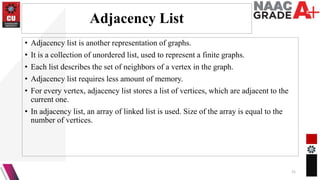
Adjacency List
• In adjacency list, an entry array[i] represents the linked list of vertices adjacent to
the ith vertex.
• Adjacency list allows to store the graph in more compact form than adjacency
matrix.
• It allows to get the list of adjacent vertices in O(1) time.
22
Fig 11: directed graph and adjacency list [5]

Disadvantages of Adjacency List
• It is not easy for adding or removing an edge to/from adjacent list.
• It does not allow to make an efficient implementation, if dynamically change of
vertices number is required.
23

Graph Traversal
Graph Traversal:
• Graph traversal is a process of checking or updating each vertex in a graph.
• It is also known as Graph Search.
• Graph traversal means visiting each and exactly one node.
• Tree traversal is a special case of graph traversal.
There are two techniques used in graph traversal:
1. Depth First Search
2. Breadth First Search
24

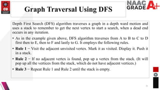
Graph Traversal Using DFS
Depth First Search (DFS) algorithm traverses a graph in a depth ward motion and
uses a stack to remember to get the next vertex to start a search, when a dead end
occurs in any iteration.
• As in the example given above, DFS algorithm traverses from A to B to C to D
first then to E, then to F and lastly to G. It employs the following rules.
• Rule 1 − Visit the adjacent unvisited vertex. Mark it as visited. Display it. Push it
in a stack.
• Rule 2 − If no adjacent vertex is found, pop up a vertex from the stack. (It will
pop up all the vertices from the stack, which do not have adjacent vertices.)
• Rule 3 − Repeat Rule 1 and Rule 2 until the stack is empty.
25

26
Fig 12: DFS Traversal [6]

27
Fig 13: DFS Traversal [7]

28
Fig 14: DFS Recursive [7]

Depth-First Search Algorithm
Step 1: SET STATUS = 1 (ready state) for each node in G
Step 2: Push the starting node A on the stack and set its STATUS = 2 (waiting state)
Step 3: Repeat Steps 4 and 5 until STACK is empty
Step 4: Pop the top node N. Process it and set its STATUS = 3 (processed state)
Step 5: Push on the stack all the neighbors of N that are in the ready state (whose
STATUS = 1) and set their STATUS = 2 (waiting state)
[END OF LOOP]
Step 6: EXIT
29

Features of Depth-First Search
• Space complexity The space complexity of a depth-first search is lower than that
of a breadth first search.
• Time complexity The time complexity of a depth-first search is proportional to the
number of vertices plus the number of edges in the graphs that are traversed. The
time complexity can be given as (O(|V| + |E|)).
• Completeness Depth-first search is said to be a complete algorithm. If there is a
solution, depth first search will find it regardless of the kind of graph. But in case
of an infinite graph, where there is no possible solution, it will diverge.
30

Applications of Depth-First Search
Following are the problems that use DFS as a building block.
1) For an unweighted graph, DFS traversal of the graph produces the minimum spanning
tree and all pair shortest path tree. DFS is at the heart of Prims and Kruskals algorithms.
2) Detecting cycle in a graph:
A graph has cycle if and only if we see a back edge during DFS. So we can run DFS for the
graph and check for back edges.
3) Path Finding:
DFS algorithm can be used to find a path between two given vertices u and z.
i) Call DFS(G, u) with u as the start vertex.
ii) Use a stack S to keep track of the path between the start vertex and the current vertex.
iii) As soon as destination vertex z is encountered, return the path as the
contents of the stack
31

Applications of Depth-First Search
4) Topological Sorting:
DFS is an intermediate step for topological sorting.
5) Finding Strongly Connected Components of a graph A directed graph is called
strongly connected if there is a path from each vertex in the graph to every other
vertex. (See this for DFS based algo for finding Strongly Connected Components)
6) DFS is very helpful in solving almost all the maze puzzles. Most of the maze
puzzles can be converted into Graph problems and traversals result into the solution.
DFS can be adapted to find all solutions to a maze by only including nodes on the
current path in the visited set.
32

Graph Traversal Using BFS
Breadth First Search (BFS) algorithm traverses a graph in a breadth ward motion
and uses a queue to remember to get the next vertex to start a search, when a dead
end occurs in any iteration.
• As in the example given above, BFS algorithm traverses from A to B to E to F first
then to C and G lastly to D. It employs the following rules.
• Rule 1 − Visit the adjacent unvisited vertex. Mark it as visited. Display it. Insert it
in a queue.
• Rule 2 − If no adjacent vertex is found, remove the first vertex from the queue.
• Rule 3 − Repeat Rule 1 and Rule 2 until the queue is empty.
33

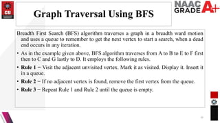
Graph Traversal Using BFS
34
Fig 15: BFS Traversal [8]

Algorithm for Breadth-First
Search
Step 1: SET STATUS = 1 (ready state) for each node in G
Step 2: Enqueue the starting node A and set its STATUS = 2 (waiting state)
Step 3: Repeat Steps 4 and 5 until QUEUE is empty
Step 4: Dequeue a node N. Process it and set its STATUS = 3 (processed state).
Step 5: Enqueue all the neighbours of N that are in the ready state (whose STATUS
= 1) and set their STATUS = 2 (waiting state)
[END OF LOOP]
Step 6: EXIT
35

BFS Example
36
Fig 16: BFS Example [9]
Consider the graph G shown in the following image, calculate the minimum path p
from node A to node E. Given that each edge has a length of 1.

Solution
Minimum Path P can be found by applying breadth first search algorithm that will begin at node A
and will end at E. the algorithm uses two queues, namely QUEUE1 and QUEUE2. QUEUE1 holds
all the nodes that are to be processed while QUEUE2 holds all the nodes that are processed and
deleted from QUEUE1.
Lets start examining the graph from Node A.
1. Add A to QUEUE1 and NULL to QUEUE2.
QUEUE1 = {A}
QUEUE2 = {NULL}
2. Delete the Node A from QUEUE1 and insert all its neighbours. Insert Node A into QUEUE2
QUEUE1 = {B, D}
QUEUE2 = {A}
3. Delete the node B from QUEUE1 and insert all its neighbours. Insert node B into QUEUE2.
QUEUE1 = {D, C, F}
QUEUE2 = {A, B}
37

Solution (Contd..)
4. Delete the node D from QUEUE1 and insert all its neighbours. Since F is the only neighbour of it
which has been inserted, we will not insert it again. Insert node D into QUEUE2.
QUEUE1 = {C, F}
QUEUE2 = { A, B, D}
5. Delete the node C from QUEUE1 and insert all its neighbours. Add node C to QUEUE2.
QUEUE1 = {F, E, G}
QUEUE2 = {A, B, D, C}
6. Remove F from QUEUE1 and add all its neighbours. Since all of its neighbours has already been
added, we will not add them again. Add node F to QUEUE2.
QUEUE1 = {E, G}
QUEUE2 = {A, B, D, C, F}
38

Solution (Contd..)
7. Remove E from QUEUE1, all of E's neighbours has already been added to QUEUE1 therefore we
will not add them again. All the nodes are visited and the target node i.e. E is encountered into
QUEUE2.
QUEUE1 = {G}
QUEUE2 = {A, B, D, C, F, E}
Now, backtrack from E to A, using the nodes available in QUEUE2.
The minimum path will be A → B → C → E.
39

Features of Breadth-First Search
• Space complexity In the breadth-first search algorithm, all the nodes at a particular level
must be saved until their child nodes in the next level have been generated. The space
complexity is therefore proportional to the number of nodes at the deepest level of the
graph. Given a graph with branching factor b (number of children at each node) and depth
d, the asymptotic space complexity is the number of nodes at the deepest level O(bd).
If the number of vertices and edges in the graph are known ahead of time, the space
complexity can also be expressed as O ( | E | + | V | ), where | E | is the total number of
edges in G and | V | is the number of nodes or vertices.
• Time complexity In the worst case, breadth-first search has to traverse through all paths to
all possible nodes, thus the time complexity of this algorithm asymptotically approaches
O(bd). However, the time complexity can also be expressed as O( | E | + | V | ), since
every vertex and every edge will be explored in the worst case.
40

Features of Breadth-First Search
• Completeness Breadth-first search is said to be a complete algorithm because if
there is a solution, breadth-first search will find it regardless of the kind of graph.
But in case of an infinite graph where there is no possible solution, it will diverge.
• Optimality Breadth-first search is optimal for a graph that has edges of equal
length, since it always returns the result with the fewest edges between the start
node and the goal node. But generally, in real-world applications, we have
weighted graphs that have costs associated with each edge, so the goal next to the
start does not have to be the cheapest goal available.
41

Applications of Breadth-First
Search
Breadth-first Search is a simple graph traversal method that has a surprising range of
applications. Here are a few interesting ways in which Bread-First Search is being
used:
• Crawlers in Search Engines: Breadth-First Search is one of the main algorithms
used for indexing web pages. The algorithm starts traversing from the source page
and follows all the links associated with the page. Here each web page will be
considered as a node in a graph.
• GPS Navigation systems: Breadth-First Search is one of the best algorithms used
to find neighboring locations by using the GPS system.
42

Graph Applications
• In Computer science graphs are used to represent the flow of computation.
• Graphs are used by Google maps for building transportation systems, where
intersection of two(or more) roads are considered to be a vertex and the road
connecting two vertices is considered to be an edge, thus their navigation system
is based on the algorithm to calculate the shortest path between two vertices.
• In Facebook, users are considered to be the vertices and if they are friends then
there is an edge running between them. Facebook’s Friend suggestion algorithm
uses graph theory.
• In Operating System, we come across the Resource Allocation Graph where each
process and resources are considered to be vertices. Edges are drawn from
resources to the allocated process, or from requesting process to the requested
resource. If this leads to any formation of a cycle then a deadlock will occur.
43

REFERENCE IMAGES
[1]https://www.tutorialspoint.com/data_structures_algorithms/graph_data_structure.ht
m
[2] http://masterraghu.com/subjects/Datastructures/ebooks/rema%20thareja.pdf
[3] https://www.tutorialride.com/data-structures/graphs-in-data-structure.htm
[4]https://www.tutorialspoint.com/data_structures_algorithms/graph_data_structure.ht
m
[6]https://www.tutorialspoint.com/data_structures_algorithms/depth_first_traversal.htm
[8]https://www.tutorialspoint.com/data_structures_algorithms/breadth_first_traversal.htm
[9]https://www.javatpoint.com/breadth-first-search-algorithm
44

REFERENCES
Reference Books:
• Seymour Lipschutz, Schaum's Outlines Series Data structures TMH
• Introduction to Data Structures Applications, Trembley & Soreson, Second
Edition, Pearson Education
Reference Links:
https://www.tutorialspoint.com/data_structures_algorithms/stack_algorithm.htm
45

THANK YOU
For queries:
Email: preeti.e8780@cumail.in

Graphs.pptx

Recommended

Recommended

More Related Content

Similar to Graphs.pptx

Similar to Graphs.pptx (20)

Recently uploaded

Recently uploaded (20)

Graphs.pptx