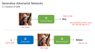
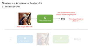
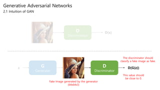
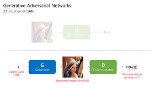
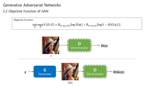
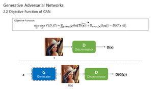
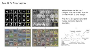
Generative adversarial networks (GANs) are a class of unsupervised machine learning models used to generate new data with the same statistics as the training set. GANs work by having two neural networks, a generator and discriminator, compete against each other. The generator tries to generate fake images that look real, while the discriminator tries to tell real images apart from fake ones. This adversarial process allows the generator to produce highly realistic images. The paper proposes GANs and introduces their objective functions and training procedure to generate images similar to samples from the training data distribution.

1. Generative Adversarial Networks
Ian J. Goodfellow, Jean Pouget-Abadie, Mehdi Mirza Machine Learning Group
University de Montreal
2014, Cited by 10479
Aug 01, 2019
SMC AI Research Center
Kyuri Kim
PR-001: Generative adversarial nets by Jaejun Yoo (2017/4/13)

2. Introduction
1.1 Supervised vs Unsupervised Learning
- Supervised Learning
- Unsupervised Learning
Variational Auto Encoder(VAE), GAN,
Clustering, Dimension Reduction, etc.
Data: (x, y)
x is data, y is label
Learn a function to map x → y
Data: (x)
Just data, no label
𝒈 𝜽(𝒙|𝒛)𝒒∅(𝒛|𝒙)

3. Introduction
1.1 Supervised vs Unsupervised Learning
- Supervised Learning
- Unsupervised Learning
Data: (x, y)
x is data, y is label
Learn a function to map x → y
mean
‘Sampling’

4. Introduction
1.1 Supervised vs Unsupervised Learning
- Supervised Learning
- Unsupervised Learning
Data: (x, y)
x is data, y is label
Learn a function to map x → y
NIPS 2016 Tutorial: generative adversarial networks paper

5. Introduction
1.2 Generative Adversarial Networks
Generated Image by Neural Network
Figure adopted from BEGAN paper released at 31. Mar.
2017, Google
- Generative Model - Adversial
Real or Fake?
Generator Discriminator
Fake
Money
Real
Money

6. Introduction
1.3 Probability Distribution
Eyeglasses Wavy Hair Wearing Hat
𝑃𝑑𝑎𝑡𝑎 𝑟𝑒𝑝𝑟𝑒𝑠𝑒𝑛𝑡𝑠 𝑡ℎ𝑒 𝑑𝑖𝑠𝑡𝑟𝑖𝑏𝑢𝑡𝑖𝑜𝑛 𝑜𝑓 𝑎𝑐𝑡𝑢𝑎𝑙 𝑖𝑚𝑎𝑔𝑒𝑠.

7. Introduction
1.3 Probability Distribution
𝐺𝑜𝑎𝑙 𝑖𝑠 𝑡𝑜 𝑓𝑖𝑛𝑑 𝑎 𝑃 𝑚𝑜𝑑𝑒𝑙 𝑡ℎ𝑎𝑡 𝑎𝑝𝑝𝑟𝑜𝑥𝑖𝑚𝑎𝑡𝑒𝑑 𝑃𝑑𝑎𝑡𝑎 𝑤𝑒𝑙𝑙.
Data Generating Distribution
Discriminator Distribution
Generative Distribution

8. Generative Adversarial Networks
2.1 Intuition of GAN
D
Discriminator
G
Generater
D
Discriminator
Real Image
Fake Image
D(x)
D(G(z))
May be High
The probability of that x came
from the real data (0~1)
May be low
z
Latent Code

9. D
Discriminator
G
Generater
D
Discriminator
D(x)
D(G(z))z
The discriminator should
classify a real image as real.
Real Image (64x64x3)
This value should be
close to 1.
Generative Adversarial Networks
2.1 Intuition of GAN

10. D
Discriminator
G
Generater
D
Discriminator
D(x)
D(G(z))
This value should
be close to 0.
z
The discriminator should
classify a fake image as fake.
Generative Adversarial Networks
2.1 Intuition of GAN
Fake Image generated by the generator
(64x64x3)

11. D
Discriminator
G
Generater
D
Discriminator
Generated Image (64x64x3)
D(x)
D(G(z))
This value should
be close to 1.
z
Latent Code
(100)
Generative Adversarial Networks
2.1 Intuition of GAN

12. Generative Adversarial Networks
2.2 Objective Function of GAN
Objective Function.
x
D
Discriminator
D(x)
G
Generater
D
Discriminator
G(z)
D(G(z))z

13. Generative Adversarial Networks
2.2 Objective Function of GAN
x
D
Discriminator
D(x)
G
Generater
D
Discriminator
G(z)
D(G(z))z
Objective Function.

14. Implementation
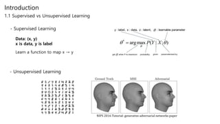
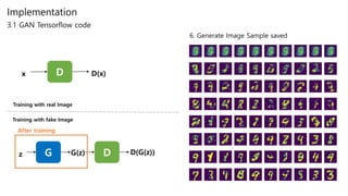
3.1 GAN Tensorflow code
mnist = input_data.read_data_sets("./mnist/data/",
one_hot=True)
total_epoch = 100
batch_size = 50
learning_rate = 0.0001
n_hidden = 256
n_input = 28 * 28
n_noise = 128
X = tf.placeholder(tf.float32, [None, n_input])
Z = tf.placeholder(tf.float32, [None, n_noise])
1. Requirements and Dataset
2. Generator Network
G_W1 = tf.Variable(tf.random_normal([n_noise, n_hidden],
stddev=0.01))
G_b1 = tf.Variable(tf.zeros([n_hidden]))
G_W2 = tf.Variable(tf.random_normal([n_hidden, n_input],
stddev=0.01))
G_b2 = tf.Variable(tf.zeros([n_input]))
def generator(noise_z):
hidden = tf.nn.relu(tf.matmul(noise_z, G_W1) + G_b1)
output = tf.nn.sigmoid(tf.matmul(hidden, G_W2) + G_b2)
return output
D D(x)x
G D D(G(z))z G(z)
Training with real Image
Training with fake Image
128
256
784
1
256784

15. Implementation
3.1 GAN Tensorflow code
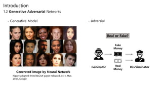
3. Discriminator Network
4. Generate Fake Image, Loss & Optimizer
D_W2 = tf.Variable(tf.random_normal([n_hidden, 1],
stddev=0.01))
D_b2 = tf.Variable(tf.zeros([1]))
def discriminator(inputs):
hidden = tf.nn.relu(tf.matmul(inputs, D_W1) + D_b1)
output = tf.nn.sigmoid(tf.matmul(hidden, D_W2) + D_b2)
return output
G = generator(Z)
D_gene = discriminator(G)
D_real = discriminator(X)
loss_D = tf.reduce_mean(tf.log(D_real) + tf.log(1 - D_gene))
loss_G = tf.reduce_mean(tf.log(D_gene))
train_D = tf.train.AdamOptimizer(learning_rate).minimize(-
loss_D, var_list=D_var_list)
train_G = tf.train.AdamOptimizer(learning_rate).minimize(-
loss_G, var_list=G_var_list)
Training with real Image
Training with fake Image
D D(x)x
G D D(G(z))z G(z)
CE(pred, y) = −y⋅log(pred)−(1−y)⋅log(1−pred)
Dloss = CE(D(x),1)+CE(D(G(z)),0) = −log(D(x))−log(1−D(g(z)) )
Gloss = CE(D(G(z)),1) = −log(D(G(z))

16. Implementation
3.1 GAN Tensorflow code
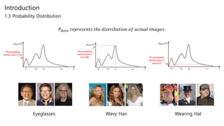
5. Training & Testing
sess = tf.Session()
sess.run(tf.global_variables_initializer())
total_batch = int(mnist.train.num_examples/batch_size)
loss_val_D, loss_val_G = 0, 0
for epoch in range(total_epoch):
for i in range(total_batch):
batch_xs, batch_ys =
mnist.train.next_batch(batch_size)
noise = get_noise(batch_size, n_noise)
# 판별기와 생성기 신경망을 각각 학습
_, loss_val_D = sess.run([train_D, loss_D],
feed_dict={X: batch_xs,
Z: noise})
_, loss_val_G = sess.run([train_G, loss_G],
feed_dict={Z: noise})
print('Epoch:', '%04d' % epoch,
'D loss: {:.4}'.format(loss_val_D),
'G loss: {:.4}'.format(loss_val_G))
Training with real Image
Training with fake Image
D D(x)x
G D D(G(z))z G(z)
noise = get_noise(sample_size, n_noise)
samples = sess.run(G, feed_dict={Z: noise})
Get Closer to 1.
Get Closer to 0.

17. Implementation
3.1 GAN Tensorflow code
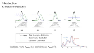
5. Training & Testing
sess = tf.Session()
sess.run(tf.global_variables_initializer())
total_batch = int(mnist.train.num_examples/batch_size)
loss_val_D, loss_val_G = 0, 0
for epoch in range(total_epoch):
for i in range(total_batch):
batch_xs, batch_ys =
mnist.train.next_batch(batch_size)
noise = get_noise(batch_size, n_noise)
# 판별기와 생성기 신경망을 각각 학습
_, loss_val_D = sess.run([train_D, loss_D],
feed_dict={X: batch_xs,
Z: noise})
_, loss_val_G = sess.run([train_G, loss_G],
feed_dict={Z: noise})
print('Epoch:', '%04d' % epoch,
'D loss: {:.4}'.format(loss_val_D),
'G loss: {:.4}'.format(loss_val_G))
Training with real Image
Training with fake Image
D D(x)x
G D D(G(z))z G(z)
noise = get_noise(sample_size, n_noise)
samples = sess.run(G, feed_dict={Z: noise})
Get Closer to 1.

18. Implementation
3.1 GAN Tensorflow code
6. Generate Image Sample saved
Training with real Image
Training with fake Image
D D(x)x
G D D(G(z))z G(z)
After training

19. Experiments
y = log(1-x) y = log(x)
The gradient is relatively small at D(G(z))=0. The gradient is very large at D(G(z))=0.
4.1 Non-Saturating game

20. Result & Conclusion
Yellow boxes are real data
samples that are nearest matches
to last column of fake images.
This shows the generator didn’t
merely memorize training
examples.