Game theory problems by an alternative simplex method

IJRET: International Journal of Research in Engineering and Technology eISSN: 2319-1163 | pISSN: 2321-7308
_______________________________________________________________________________________
Volume: 03 Issue: 05 | May-2014, Available @ http://www.ijret.org 900
GAME THEORY PROBLEMS BY AN ALTERNATIVE SIMPLEX
METHOD
Kirtiwant P. Ghadle1
, Tanaji S. Pawar2
1
Associate Professor, Department of Mathematics, Dr. Babasaheb Ambedkar Marathwada University, Aurangabad,
Maharashtra, India
2
Research Student, Department of Mathematics, Dr. Babasaheb Ambedkar Marathwada University, Aurangabad,
Maharashtra, India
Abstract
In this paper, an alternative method for the solution of game problems is introduced. This method is easy to solve game problem
which does not have a saddle point. It is powerful method to reduce number of iterations and save valuable time.
Keywords: Linear programming problem, Optimal solution, Alternative simplex method, and Game problem.
--------------------------------------------------------------------***------------------------------------------------------------------
1. INTRODUCTION
Today’s life is a full of struggle and competitions. A great
variety of competitive situations is commonly seen. What
should be the bid to win a big government job in the pace of
competition from several jobs? Game must be thought of, in
abroad sense, not as a kind of sport but as competitive
situation, a kind of conflict in which somebody must win
and somebody must lose.
John Von Neumann suggestion is to solve the game theory
problems on the maximum losses. Dantzig [1] suggestion is
to choose that entering vector corresponding to which
𝑧𝑗 − 𝑐𝑗 is most negative. Khobragade et al. [2, 3, 4]
suggestion is to choose that entering vector corresponding to
which
( 𝑧 𝑗 − 𝑐 𝑗 ) 𝜃 𝑗
𝑐 𝑗
is most negative.
In this paper, an attempt has been made to solve linear
programming problem (LPP) by new method which is an
alternative for simplex method. This method is different
from Khobragade et al. Method.
2. SOLUTION OF M x N RECTANGULAR
GAME PROBLEM
By fundamental theorem of rectangular games, if mixed
strategies are allowed, there always exists a value of game.
( i.e. 𝑉 = 𝑉 = 𝑉 ).
Let the two person zero sum game be defined as follows:
Player B
Player A
𝑎11 ⋯ 𝑎1𝑛
⋮ ⋱ ⋮
𝑎 𝑚1 ⋯ 𝑎 𝑚𝑛
Let 𝑝1, 𝑝2, … , 𝑝 𝑚 and 𝑞1, 𝑞2, … , 𝑞 𝑛 be the probabilities of
two players A and B, to select their pure strategies. i.e.
𝑆𝐴 = 𝑝1, 𝑝2, … , 𝑝 𝑚 and 𝑆 𝐵 = (𝑞1, 𝑞2, … , 𝑞 𝑛 ).
Then 𝑝1 + 𝑝2 + 𝑝3 + … + 𝑝 𝑚 = 1
and 𝑞1 + 𝑞2 + 𝑞3 + … + 𝑞 𝑛 = 1,
Where 𝑝𝑖 ≥ 0 and 𝑞𝑗 ≥ 0 for all 𝑖, 𝑗.
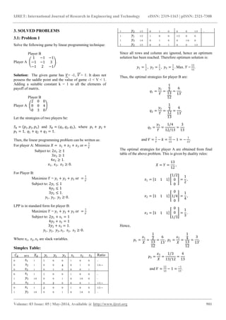
Let the game can be defined by LPP as given below:
For player A: Minimize 𝑋 = 𝑥1 + 𝑥2 + ⋯ + 𝑥 𝑚 or =
1
𝑉
Subject to: 𝑎11 𝑥1 + 𝑎21 𝑥2 + ⋯ + 𝑎 𝑚1 𝑥 𝑚 ≥ 1
𝑎12 𝑥1 + 𝑎22 𝑥2 + ⋯ + 𝑎 𝑚2 𝑥 𝑚 ≥ 1
..................................................
..................................................
𝑎1𝑛 𝑥1 + 𝑎2𝑛 𝑥2 + ⋯ + 𝑎 𝑚𝑛 𝑥 𝑚 ≥ 1
𝑥1, 𝑥2, … , 𝑥 𝑚 ≥ 0.
For Player B: Maximize 𝑌 = 𝑦1 + 𝑦2 + ⋯ + 𝑦𝑛 or =
1
𝑉
Subject to: 𝑎11 𝑦1 + 𝑎12 𝑦2 + ⋯ + 𝑎1𝑛 𝑦 𝑚 ≤ 1
𝑎21 𝑦1 + 𝑎22 𝑦2 + ⋯ + 𝑎2𝑛 𝑦 𝑚 ≤ 1
..................................................
..................................................
𝑎 𝑚1 𝑦1 + 𝑎 𝑚2 𝑦2 + ⋯ + 𝑎 𝑚𝑛 𝑦 𝑚 ≤ 1
𝑥1, 𝑥2, … , 𝑥 𝑚 ≥ 0.
To find the optimal solution of the above LPP, it has been
observed that the player B’s problem is exactly the dual of
the player A’s problem. The optimal solution of one
problem will automatically give the optimal solution to the
other. The player B’s problem can be solved by an
alternative simplex method while player A’s problem can be
solved by an alternative dual simplex method [7].

_______________________________________________________________________________________
3. SOLVED PROBLEMS
3.1: Problem 1
Solve the following game by linear programming technique:
Player B
Player A
1 −1 −1
−1 −1 3
−1 2 −1
.
Solution: The given game has 𝑉= -1, 𝑉 = 1. It does not
possess the saddle point and the value of game -1 < V < 1.
Adding a suitable constant k = 1 to all the elements of
payoff of matrix.
Player B
Player A
2 0 0
0 0 4
0 3 0
Let the strategies of two players be:
𝑆𝐴 = 𝑝1, 𝑝2, 𝑝3 and 𝑆 𝐵 = (𝑞1, 𝑞2, 𝑞3), where 𝑝1 + 𝑝2 +
𝑝3 = 1, 𝑞1 + 𝑞2 + 𝑞3 = 1.
Then, the linear programming problem can be written as:
For player A: Minimize 𝑋 = 𝑥1 + 𝑥2 + 𝑥3 or =
1
𝑉
Subject to: 2𝑥1 ≥ 1
3𝑥3 ≥ 1
4𝑥2 ≥ 1.
𝑥1, 𝑥2, 𝑥3 ≥ 0.
For Player B:
Maximize 𝑌 = 𝑦1 + 𝑦2 + 𝑦3 or =
1
𝑉
Subject to: 2𝑦1 ≤ 1
4𝑦3 ≤ 1
3𝑦2 ≤ 1.
𝑦1, 𝑦2, 𝑦3 ≥ 0.
LPP is in standard form for player B:
1
𝑉
Subject to: 2𝑦1 + 𝑠1 = 1
4𝑦3 + 𝑠2 = 1
3𝑦2 + 𝑠3 = 1.
𝑦1, 𝑦2, 𝑦3, 𝑠1, 𝑠2, 𝑠3 ≥ 0.
Where 𝑠1, 𝑠2, 𝑠3 are slack variables.
Simplex Table:
𝐶 𝐵 BVS 𝑋 𝐵 𝑦1 𝑦2 𝑦3 𝑠1 𝑠2 𝑠3 Ratio
0 𝑠1 1 2 0 0 1 0 0 -
0 𝑠2 1 0 0 4 0 1 0 1/4→
0 𝑠3 1 0 3 0 0 0 1 -
0 𝑠1 1 2 0 0 1 0 0 -
1 𝑦3 1/4 0 0 1 0 1/4 0 -
0 𝑠3 1 0 3 0 0 0 1 1/3→
0 𝑠1 1 2 0 0 1 0 0 1/2→
1 𝑦3 1/4 0 0 1 0 1/4 0 -
1 𝑦2 1/3 0 1 0 0 0 1/3 -
1 𝑦1 1/2 1 0 0 1/2 0 0
1 𝑦3 1/4 0 1 0 0 1/4 0
1 𝑦2 1/3 0 0 1 0 0 1/3
Since all rows and column are ignored, hence an optimum
solution has been reached. Therefore optimum solution is:
𝑦1 =
1
2
, 𝑦2 =
1
3
, 𝑦3 =
1
4
. Max. 𝑌 =
13
12
.
Thus, the optimal strategies for player B are:
𝑞1 =
𝑦1
𝑌
=
1
2
13
12
=
6
13
,
𝑞2 =
𝑦2
𝑌
=
1
3
12
13
=
4
13
,
𝑞3 =
𝑦3
𝑌
=
1/4
12/13
=
3
13
and 𝑉 =
1
𝑌
− 𝑘 =
12
13
− 1 = −
1
13
.
The optimal strategies for player A are obtained from final
table of the above problem. This is given by duality rules:
𝑋 = 𝑌 =
13
12
,
𝑥1 = 1 1 1
1/2
0
0
=
1
2
,
𝑥2 = 1 1 1
0
1/4
0
=
1
4
,
𝑥3 = 1 1 1
0
0
1/3
=
1
3
.
Hence,
𝑝1 =
𝑥1
𝑋
=
1
2
13
12
=
6
13
, 𝑝2 =
𝑥2
𝑋
=
1
4
13
12
=
3
13
,
𝑝3 =
𝑥3
𝑋
=
1/3
13/12
=
4
13
and 𝑉 =
12
13
− 1 =
−1
13
.

_______________________________________________________________________________________
3.2: Problem 2:
Two companies P and Q are competing for the same
product. Their different strategies are given in the following
payoff matrix:
Player Q
Player P
1 2 4
2 2 1
3 1 1
.
Use linear programming to determine the best strategies for
both the companies.
Solution: The given game has 𝑉= 1, 𝑉 = 2. It does not
possess the saddle point and the value of game 1 < V < 2.
Here, the payoff matrix is already non-negative.
𝑝3 = 1, 𝑞1 + 𝑞2 + 𝑞3 = 1.
For player A:
Minimize 𝑋 = 𝑥1 + 𝑥2 + 𝑥3 or =
1
𝑉
Subject to: 𝑥1 + 2𝑥2 + 3𝑥3 ≥ 1
2𝑥1 + 2𝑥2 + 𝑥3 ≥ 1
4𝑥1 + 𝑥2 + 𝑥3 ≥ 1.
𝑥1, 𝑥2, 𝑥3 ≥ 0.
For Player B:
1
𝑉
Subject to: 𝑦1 + 2𝑦2 + 4𝑦3 ≤ 1
2𝑦1 + 2𝑦2 + 𝑦3 ≤ 1
3𝑦1 + 𝑦2 + 𝑦3 ≤ 1.
𝑦1, 𝑦2, 𝑦3 ≥ 0.
1
𝑉
Subject to: 𝑦1 + 2𝑦2 + 4𝑦3 + 𝑠1 = 1
2𝑦1 + 2𝑦2 + 𝑦3 + 𝑠2 = 1
3𝑦1 + 𝑦2 + 𝑦3 + 𝑠3 = 1.
𝑦1, 𝑦2, 𝑦3, 𝑠1, 𝑠2, 𝑠3 ≥ 0.
Where 𝑠1, 𝑠2, 𝑠3 are slack variables.
Simplex Table:
𝐶 𝐵 BVS 𝑋 𝐵 𝑦1 𝑦2 𝑦3 𝑠1 𝑠2 𝑠3 Ratio
0 𝑠1 1 1 2 4 1 0 0 1/4→
0 𝑠2 1 2 2 1 0 1 0 1
0 𝑠3 1 3 1 1 0 0 1 1
1 𝑦3 1/4 1/4 1/2 1 1/2 0 0
0 𝑠2 3/4 7/4 3/2 0 -1/4 1 0 3/7
0 𝑠3 3/4 11/4 1/2 0 -1/4 0 1 3/11→
1 𝑦3 2/11 0 5/11 1 3/11 0 -
1/11
0 𝑠2 3/11 0 13/11 0 -
1/11
1 -
7/11
3/13→
1 𝑦1 3/11 1 2/11 0 -
1/11
0 4/11
1 𝑦3 1/13 0 0 1 4/13 -5/13 2/13
1 𝑦2 3/13 0 1 0 -
1/13
11/13 -
7/13
1 𝑦1 3/13 1 0 0 -
1/13
-2/13 6/13
𝑦1 =
3
13
, 𝑦2 =
3
13
, 𝑦3 =
1
13
. Max. 𝑌 =
7
13
.
𝑞1 =
𝑦1
𝑌
=
3
13
7
13
=
3
7
,
𝑞2 =
𝑦2
𝑌
=
3
13
7
13
=
3
7
,
𝑞3 =
𝑦3
𝑌
=
1/13
7/13
=
1
7
and 𝑉 =
1
𝑌
− 𝑘 =
13
7
− 0 =
13
7
.
𝑋 = 𝑌 =
7
13
,
𝑥1 = 1 1 1
4/13
−1/13
−1/13
=
2
13
,
𝑥2 = 1 1 1
−5/13
11/13
−2/13
=
4
13
,
𝑥3 = 1 1 1
2/13
−7/13
6/13
=
1
13
.
Hence,
𝑝1 =
𝑥1
𝑋
=
2
13
7
13
=
2
7
, 𝑝2 =
𝑥2
𝑋
=
4
13
7
13
=
4
7
,
𝑝3 =
𝑥3
𝑋
=
1/13
7/13
=
1
7
and 𝑉 =
13
7
− 0 =
13
7
.

_______________________________________________________________________________________
3.3: Problem 3:
Solve the following game by linear programming technique:
Player B
Player A
3 −1 −3
−3 3 −1
−4 −3 3
.
To make this payoff matrix as positive, adding a suitable
constant k = 5 to all the elements of payoff of matrix.
Player B
Player A
8 4 2
2 8 4
1 2 8
𝑝3 = 1, 𝑞1 + 𝑞2 + 𝑞3 = 1.
1
𝑉
Subject to: 8𝑥1 + 2𝑥2 + 𝑥3 ≥ 1
4𝑥1 + 8𝑥2 + 2𝑥3 ≥ 1
2𝑥1 + 4𝑥2 + 8𝑥3 ≥ 1.
𝑥1, 𝑥2, 𝑥3 ≥ 0.
For Player B:
1
𝑉
Subject to: 8𝑦1 + 4𝑦2 + 3𝑦3 ≤ 1
2𝑦1 + 8𝑦2 + 4𝑦3 ≤ 1
𝑦1 + 2𝑦2 + 8𝑦3 ≤ 1.
𝑦1, 𝑦2, 𝑦3 ≥ 0.
Maximize 𝑌 = 𝑦1 + 𝑦2 + 𝑦3
Subject to: 8𝑦1 + 4𝑦2 + 3𝑦3 + 𝑠1 = 1
2𝑦1 + 8𝑦2 + 4𝑦3 + 𝑠2 = 1
𝑦1 + 2𝑦2 + 8𝑦3 + 𝑠3 = 1.
𝑦1, 𝑦2, 𝑦3, 𝑠1, 𝑠2, 𝑠3 ≥ 0.
where 𝑠1, 𝑠2, 𝑠3 are slack variables.
Simplex Table:
𝐶 𝐵 B
V
S
𝑋 𝐵 𝑦1 𝑦2 𝑦3 𝑠1 𝑠2 𝑠3 Ratio
0 𝑠1 1 8 4 2 1 0 0 1/8→
0 𝑠2 1 2 8 4 0 1 0 1/2
0 𝑠3 1 1 2 8 0 0 1 1
1 𝑦1 1/8 1 1/2 1/4 1/8 0 0
0 𝑠2 3/4 0 7 7/2 -1/4 1 0 3/14
0 𝑠3 7/8 0 3/2 31/4 -1/8 0 1 7/62→
1 𝑦1 3/31 1 14/31 0 4/31 0 -1/31
0 𝑠2 11/31 0 196/31 0 -6/31 1 - 11/196
14/31 →
1 𝑦3 7/62 0 6/31 1 -1/62 0 4/31
1 𝑦1 1/14 1 0 0 1/7 -1/14 0
1 𝑦2 11/196 0 1 0 -3/98 31/196 -1/14
1 𝑦3 5/49 0 0 1 -1/98 -3/98 1/7
𝑦1 =
1
14
, 𝑦2 =
11
196
, 𝑦3 =
5
49
. Max. 𝑌 =
45
196
.
𝑞1 =
𝑦1
𝑌
=
1
14
45
196
=
14
45
,
𝑞2 =
𝑦2
𝑌
=
11
196
45
196
=
11
45
,
𝑞3 =
𝑦3
𝑌
=
5/49
45/196
=
20
45
and 𝑉 =
1
𝑌
− 𝑘 =
196
45
− 5 = −
29
45
.
𝑋 = 𝑌 =
45
196
,
𝑥1 = 1 1 1
1/7
−3/98
−1/98
=
5
49
,
𝑥2 = 1 1 1
−1/14
31/196
−3/98
=
11
196
,
𝑥3 = 1 1 1
0
−1/14
1/7
=
1
14
.
Hence,
𝑝1 =
𝑥1
𝑋
=
5
49
45
196
=
20
45
, 𝑝2 =
𝑥2
𝑋
=
11
196
45
196
=
11
45
,
𝑝3 =
𝑥3
𝑋
=
1/14
45/196
=
14
45
and 𝑉 =
196
45
− 5 = −
29
45
.

_______________________________________________________________________________________
3.4: Problem 4:
Two companies P and Q are competing for the same
product. Their different strategies are given in the following
payoff matrix:
Player Q
Player P
−1 0 2
0 0 −1
1 −1 −1
.
Use linear programming to determine the best strategies for
both the companies.
To make this payoff matrix as positive, adding a suitable
constant k = 2 to all the elements of payoff of matrix.
Player B
Player A
1 2 4
2 2 1
3 1 1
𝑝3 = 1, 𝑞1 + 𝑞2 + 𝑞3 = 1.
1
𝑉
Subject to: 𝑥1 + 2𝑥2 + 3𝑥3 ≥ 1
2𝑥1 + 2𝑥2 + 𝑥3 ≥ 1
4𝑥1 + 𝑥2 + 𝑥3 ≥ 1.
𝑥1, 𝑥2, 𝑥3 ≥ 0.
Min. 𝑍 = - Max. −𝑍 , −𝑍 = 𝑍∗
Max. 𝑍∗
= −𝑥1 − 𝑥2 − 𝑥3
Subject to: −𝑥1 − 2𝑥2 − 3𝑥3 ≤ −1
−2𝑥1 − 2𝑥2 − 𝑥3 ≤ −1
−4𝑥1 − 𝑥2 − 𝑥3 ≤ −1.
𝑥1, 𝑥2, 𝑥3 ≥ 0.
LPP is in standard form for player A:
Max. 𝑍∗
= 𝑥1 − 𝑥2 − 𝑥3
Subject to: −𝑥1 − 2𝑥2 − 3𝑥3 + 𝑠1 = −1
−2𝑥1 − 2𝑥2 − 𝑥3 + 𝑠2 = −1
−4𝑥1 − 𝑥2 − 𝑥3 + 𝑠3 = −1
𝑥1, 𝑥2, 𝑥3, 𝑠1, 𝑠2, 𝑠3 ≥ 0.
where 𝑠1, 𝑠2, 𝑠3 are slack variables.
Simplex Table:
𝐶 𝐵 BVS 𝑋 𝐵 𝑥1 𝑥2 𝑥3 𝑠1 𝑠2 𝑠3 Ratio
0 𝑠1 -1 -1 -2 -3 1 0 0 1
0 𝑠2 -1 -2 -2 -1 0 1 0 1/2
0 𝑠3 -1 -4 -1 -1 0 0 1 1/4→
0 𝑠1 -3/4 0 -7/4 -
11/4
1 0 -1/4
0 𝑠2 -1/2 0 -3/2 -1/2 0 0 -1/2
-1 𝑥1 1/4 1 1/4 1/4 0 1 -1/4
-1 𝑥3 3/11 0 7/11 1 -4/11 0 1/11
0 𝑠2 -4/11 0 -
13/11
0 -2/11 1 -5/11
-1 𝑥1 2/11 1 1/11 0 1/11 0 -3/11
-1 𝑥3 1/13 0 0 1 -6/13 7/13 -2/13
-1 𝑥2 4/13 0 1 0 2/13 -
11/13
5/13
-1 𝑥1 2/13 1 0 0 1/13 1/13 -4/13
𝑥1 =
2
13
, 𝑥2 =
4
13
, 𝑥3 =
1
13
. Min. 𝑋 =
7
13
.
Thus, the optimal strategies for player A are:
𝑝1 =
𝑥1
𝑋
=
2
13
7
13
=
2
7
, 𝑝2 =
𝑥2
𝑋
=
4
13
7
13
=
4
7
,
𝑝3 =
𝑥3
𝑋
=
1/13
7/13
=
1
7
and =
1
𝑋
− 𝑘 =
13
7
− 2 = −
1
7
.
The optimal strategies for player B are obtained from final
𝑋 = 𝑌 =
7
13
,
𝑦1 = −1 −1 −1
−6/13
2/13
1/13
=
3
13
,
𝑦2 = −1 −1 −1
7/13
−11/13
1/13
=
3
13
,
𝑦3 = −1 −1 −1
−2/13
5/13
−4/13
=
1
13
.
Hence,
𝑞1 =
𝑦1
𝑌
=
3
13
7
13
=
3
7
, 𝑞2 =
𝑦2
𝑌
=
3
13
7
13
=
3
7
,
𝑞3 =
𝑦3
𝑌
=
1/13
7/13
=
1
7
and 𝑉 =
13
7
− 2 = −
1
7
.

_______________________________________________________________________________________
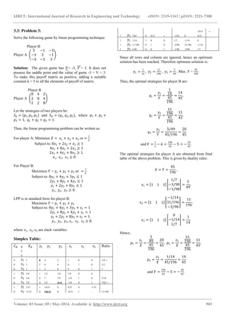
4. CONCLUSIONS
An alternative method for game theory problems to obtain
the solution of linear programming problem has been
derived. This technique is useful to apply on numerical
problems, reduces the labour work and save valuable time.
REFERENCES
[1]. G. B. Dantzig: Maximization of linear function of
variables subject to linear inequalities, In: 21-Ed. Koopman
Cowls Commission Monograph, 13, John Wiley and Sons,
Inc., New Yark (1951).
[2]. K. G. Lokhande, N. W. Khobragade, P. G. Khot:
Simplex Method: An Alternative Approach, International
Journal of Engineering and Innovative Technology, Volume
3, Issue 1, P: 426-428 (2013).
[3]. N. V. Vaidya, N. W. Khobragade: Solution of Game
Problems Using New Approach, IJEIT, Vol. 3, Issue 5,
2013.
[4]. N. W. Khobragade and P. G. Khot: Alternative
Approach to the Simplex Method-II, Acta Ciencia Indica,
Vol.xxx IM, No.3, 651, India (2005).
[5]. S. D. Sharma: Operation Research, Kedar Nath Ram
Nath, 132, R. G. Road, Meerut-250001 (U.P.), India.
[6]. S. I. Gass: Linear Programming, 3/e, McGraw-Hill
Kogakusha, Tokyo (1969).
[7]. K. P. Ghadle, T. S. Pawar, N. W. Khobragade: Solution
of Linear Programming Problem by New Approach, IJEIT,
Vol.3, Issue 6. Pp.301-307, 2013
BIOGRAPHIES
Mr. Tanaji S. Pawar, Research student,
Department of mathematics, Dr. Babasaheb
Ambedkar Marathwada University,
Aurangabad.
Dr. K. P. Ghadle for being M.Sc in Maths he
attained Ph.D. He has been teaching since
1996. At present he is working as Associate
Professor. Achieved excellent experiences in
Research for 15 years in the area of Boundary
value problems and its application. Published more than 45
research papers in reputed journals. Four students awarded
Ph.D Degree and four students working for award of Ph.D.
Degree under their guidance.

Game theory problems by an alternative simplex method

More Related Content

What's hot

Viewers also liked

Similar to Game theory problems by an alternative simplex method

More from eSAT Publishing House

Recently uploaded

Game theory problems by an alternative simplex method