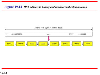
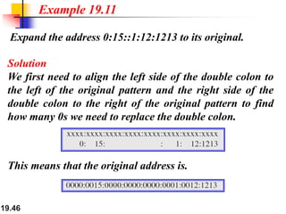
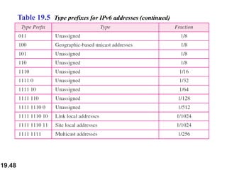
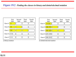
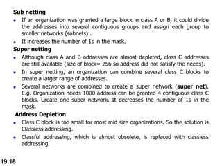
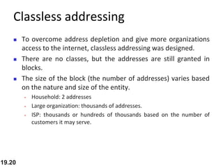
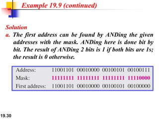
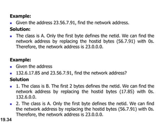
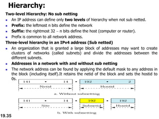
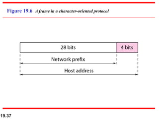
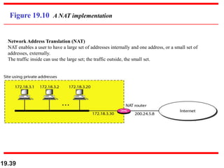
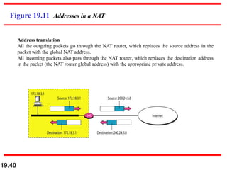
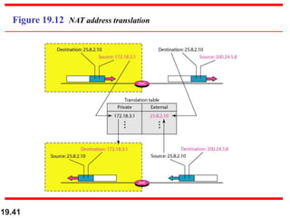
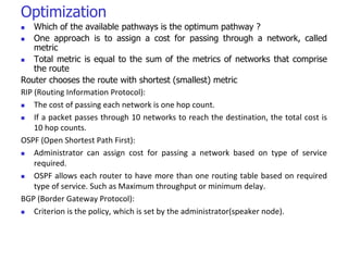
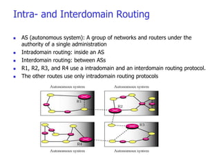
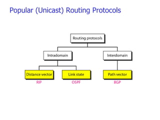
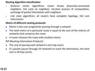
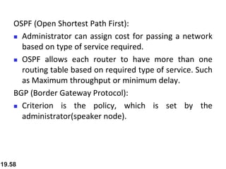
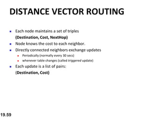
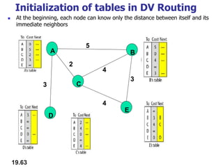
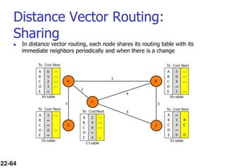
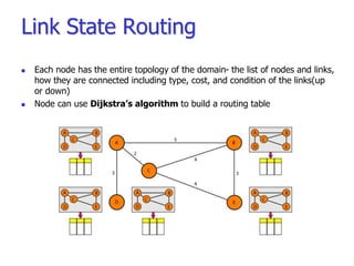
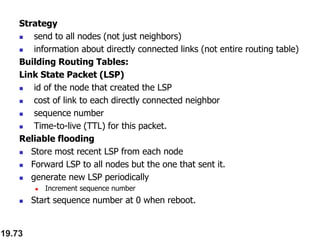
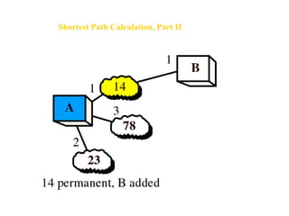
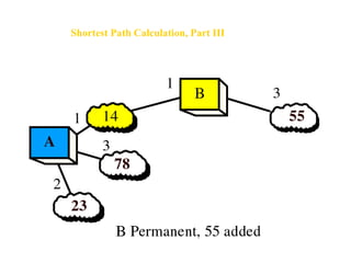
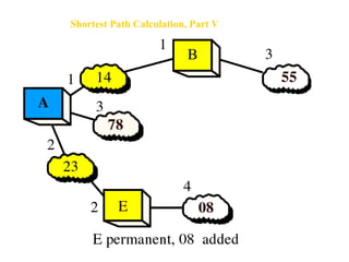
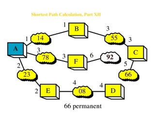
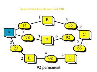
This document discusses IPv4 and IPv6 addressing and routing. It covers topics such as: - IPv4 addresses are 32-bit and unique, while IPv6 addresses are 128-bit - Classful and classless addressing in IPv4, including network masks - Network address translation (NAT) allows private addresses to connect to the public internet - Routing protocols like RIP, OSPF, and BGP are used for intradomain and interdomain routing based on metrics and shortest paths - IPv6 was developed to address the long-term address depletion problem in IPv4

1. 19.1
Network Layer:
Logical Addressing

2. 19.2
19-1 IPv4 ADDRESSES
An IPv4 address is a 32-bit address that uniquely and
universally defines the connection of a device (for
example, a computer or a router) to the Internet.
Address Space
Notations
Classful Addressing
Classless Addressing
Network Address Translation (NAT)

3. 19.3
An IPv4 address is 32 bits long.
Note

4. 19.4
The IPv4 addresses are unique
and universal.
Note

5. 19.5
The address space of IPv4 is
232 or 4,294,967,296.
Note

6. 19.6
Figure 19.1 Dotted-decimal notation and binary notation for an IPv4 address

7. Example 19.1
Change the following IP addresses from binary notation to dotted-decimal notation.
a. 10000001 00001011 00001011 11101111
b. 11111001 10011011 11111011 00001111
Solution
We replace each group of 8 bits with its equivalent decimal number and add dots for
separation:
a. 129.11.11.239
b. 249.155.251.15

8. Example 19.2
Change the following IP addresses from dotted-decimal notation to binary notation.
a. 111.56.45.78
b. 75.45.34.78
Solution
We replace each decimal number with its binary equivalent :
a. 01101111 00111000 00101101 01001110
b. 01001011 00101101 00100010 01001110

9. Types of Addressing
There are two type of addressing. They are
 Classful addressing
 Classless addressing
19.9

10. 19.10
In classful addressing, the address
space is divided into five classes:
A, B, C, D, and E.
Note

11. 19.11
Figure 19.2 Finding the classes in binary and dotted-decimal notation

12.  Class A address: designed for large organizations with a large number of attached
hosts or routers. (Wasted and not used)
 Class B address: designed for midsize organizations with tens of thousands of
attached hosts or routers (too large for many organizations)
 Class C address: designed for small organizations with a small number of attached
hosts or routers. (too small for many organizations)
 Class D address: designed for multicasting. (Waste of addresses)
 Class E address: reserved for future use (waste of addresses)
The following IP address ranges belong to Google:
 64.233.160.0 - 64.233.191.255
 66.102.0.0 - 66.102.15.255
 66.249.64.0 - 66.249.95.255
 72.14.192.0 - 72.14.255.255
 74.125.0.0 - 74.125.255.255
 209.85.128.0 - 209.85.255.255
 216.239.32.0 - 216.239.63.255
Netid and Hostid
 The address is divided into netid and hostid.
 These parts are of varying lengths, depending on the class.
19.12

13. Blocks in class A
19.13

14. 19.14
In classful addressing, a large part of the
available addresses were wasted.
Note

15. 19.15
Find the class of each address.
a. 00000001 00001011 00001011 11101111
b. 11000001 10000011 00011011 11111111
c. 14.23.120.8
d. 252.5.15.111
Example 19.4
Solution
a. The first bit is 0. This is a class A address.
b. The first 2 bits are 1; the third bit is 0. This is a class C
address.
c. The first byte is 14; the class is A.
d. The first byte is 252; the class is E.

16. 19.16
Table 19.1 Number of blocks and block size in classful IPv4 addressing

17. Mask
 It can help us to find the netid and hostid.
 It is 32-bit number made of contiguous 1s followed by contiguous 0s.
CIDR (Classless Interdomain Routing) or slash notation:
 It is used to show the mask in the form /n (n=8, 16, 24)
 In classful addressing, a large part of the available addresses were wasted.
19.17
Table 19.2 Default masks for classful addressing

18. Sub netting
 If an organization was granted a large block in class A or B, it could divide
the addresses into several contiguous groups and assign each group to
smaller networks (subnets) .
 It increases the number of 1s in the mask.
Super netting
 Although class A and B addresses are almost depleted, class C addresses
are still available (size of block= 256 so address did not satisfy the needs).
 In super netting, an organization can combine several class C blocks to
create a larger range of addresses.
 Several networks are combined to create a super network (super net).
E.g. Organization needs 1000 address can be granted 4 contiguous class C
blocks. Create one super network. It decreases the number of 1s in the
mask.
Address Depletion
 Class C block is too small for most mid size organizations. So the solution is
Classless addressing.
 Classful addressing, which is almost obsolete, is replaced with classless
addressing.
19.18

19. 19.19
Classful addressing, which is almost
obsolete, is replaced with classless
addressing.
Note

20. Classless addressing
 To overcome address depletion and give more organizations
access to the internet, classless addressing was designed.
 There are no classes, but the addresses are still granted in
blocks.
 The size of the block (the number of addresses) varies based
on the nature and size of the entity.
• Household: 2 addresses
• Large organization: thousands of addresses.
• ISP: thousands or hundreds of thousands based on the number of
customers it may serve.
19.20

21. 19.21
Figure 19.3 A block of 16 addresses granted to a small organization

22. 19.22
In IPv4 addressing, a block of
addresses can be defined as
x.y.z.t /n
in which x.y.z.t defines one of the
addresses and the /n defines the mask.
Note

23. 19.23
The first address in the block can be
found by setting the rightmost
32 − n bits to 0s.
Note

24. 19.24
A block of addresses is granted to a small organization.
We know that one of the addresses is 205.16.37.39/28.
What is the first address in the block?
Solution
The binary representation of the given address is
11001101 00010000 00100101 00100111
If we set 32−28 rightmost bits to 0, we get
11001101 00010000 00100101 0010000
or
205.16.37.32.
This is actually the block shown in Figure 19.3.
Example 19.6

25. 19.25
The last address in the block can be
found by setting the rightmost
32 − n bits to 1s.
Note

26. 19.26
Find the last address for the block in Example 19.6.
Solution
The binary representation of the given address is
11001101 00010000 00100101 00100111
If we set 32 − 28 rightmost bits to 1, we get
11001101 00010000 00100101 00101111
or
205.16.37.47
This is actually the block shown in Figure 19.3.
Example 19.7

27. 19.27
The number of addresses in the block
can be found by using the formula
232−n.
Note

28. 19.28
Find the number of addresses in Example 19.6.
Example 19.8
Solution
The value of n is 28, which means that number
of addresses is 2 32−28 or 16.

29. 19.29
Another way to find the first address, the last address, and
the number of addresses is to represent the mask as a 32-
bit binary (or 8-digit hexadecimal) number. This is
particularly useful when we are writing a program to find
these pieces of information. In Example 19.5 the /28 can
be represented as
11111111 11111111 11111111 11110000
(twenty-eight 1s and four 0s).
Find
a. The first address
b. The last address
c. The number of addresses.
Example 19.9

30. 19.30
Solution
a. The first address can be found by ANDing the given
addresses with the mask. ANDing here is done bit by
bit. The result of ANDing 2 bits is 1 if both bits are 1s;
the result is 0 otherwise.
Example 19.9 (continued)

31. 19.31
b. The last address can be found by ORing the given
addresses with the complement of the mask. ORing
here is done bit by bit. The result of ORing 2 bits is 0 if
both bits are 0s; the result is 1 otherwise. The
complement of a number is found by changing each 1
to 0 and each 0 to 1.
Example 19.9 (continued)

32. 19.32
c. The number of addresses can be found by
complementing the mask, interpreting it as a decimal
number, and adding 1 to it.
Example 19.9 (continued)

33. 19.33
NETWORK ADDRESS:
The first address in a block is normally not
assigned to any device; it is used as the network
address that represents the organization to the
rest of the world.
Note

34. Example:
 Given the address 23.56.7.91, find the network address.
Solution:
 The class is A. Only the first byte defines the netid. We can find the
network address by replacing the hostid bytes (56.7.91) with 0s.
Therefore, the network address is 23.0.0.0.
Example:
 Given the address
 132.6.17.85 and 23.56.7.91, find the network address?
Solution
 1. The class is B. The first 2 bytes defines the netid. We can find the
network address by replacing the hostid bytes (17.85) with 0s.
132.6.0.0.
 2. The class is A. Only the first byte defines the netid. We can find
the network address by replacing the hostid bytes (56.7.91) with 0s.
Therefore, the network address is 23.0.0.0.
19.34

35. Hierarchy:
Two-level Hierarchy: No sub netting
 An IP address can define only two levels of hierarchy when not sub netted.
 Prefix: the leftmost n bits define the network
 Suffix: the rightmost 32  n bits define the host (computer or router).
 Prefix is common to all network address.
Three-level hierarchy in an IPv4 address (Sub netted)
 An organization that is granted a large block of addresses may want to create
clusters of networks (called subnets) and divide the addresses between the
different subnets.
 Addresses in a network with and without sub netting
 The network address can be found by applying the default mask to any address in
the block (including itself).It retains the netid of the block and sets the hostid to
0s.
19.35

36. 19.36
Figure 19.5 Two levels of hierarchy in an IPv4 address
IP address, like other address, has levels of hierarchy.
For example: telephone network in North America

37. 19.37
Figure 19.6 A frame in a character-oriented protocol

38. 19.38
Figure 19.8 Three-level hierarchy in an IPv4 address

39. 19.39
Figure 19.10 A NAT implementation
Network Address Translation (NAT)
NAT enables a user to have a large set of addresses internally and one address, or a small set of
addresses, externally.
The traffic inside can use the large set; the traffic outside, the small set.

40. 19.40
Figure 19.11 Addresses in a NAT
Address translation
All the outgoing packets go through the NAT router, which replaces the source address in the
packet with the global NAT address.
All incoming packets also pass through the NAT router, which replaces the destination address
in the packet (the NAT router global address) with the appropriate private address.

41. 19.41
Figure 19.12 NAT address translation

42. 19.42
19-2 IPv6 ADDRESSES
Despite all short-term solutions, address depletion is
still a long-term problem for the Internet. This and
other problems in the IP protocol itself have been the
motivation for IPv6.
Structure
Address Space
Topics discussed in this section:

43. 19.43
An IPv6 address is 128 bits long.
Note

44. 19.44
Figure 19.14 IPv6 address in binary and hexadecimal colon notation

45. 19.45
Figure 19.15 Abbreviated IPv6 addresses

46. 19.46
Expand the address 0:15::1:12:1213 to its original.
Example 19.11
Solution
We first need to align the left side of the double colon to
the left of the original pattern and the right side of the
double colon to the right of the original pattern to find
how many 0s we need to replace the double colon.
This means that the original address is.

47. 19.47
Table 19.5 Type prefixes for IPv6 addresses

48. 19.48
Table 19.5 Type prefixes for IPv6 addresses (continued)

49. 19.49
Figure 19.16 Prefixes for provider-based unicast address

50. 19.50
Figure 19.17 Multicast address in IPv6

51. 19.51
Figure 19.18 Reserved addresses in IPv6

52. 19.52
Figure 19.19 Local addresses in IPv6

53. Routing Table
 Static routing table: created manually
 Dynamic routing table: updated periodically by using one of the dynamic
routing protocols such as RIP, OSPF, or BGP.
Routing Protocols
 A router consults a routing table when a packet is ready to be forwarded
 The routing table specifies the optimum path for the packet: static or
dynamic
 Internet needs dynamic routing tables to be updated as soon as there is a
change
 There are two routing: Unicast routing and multicasting routing
 RIP (Routing Information Protocol), OSPF (Open Shortest Path First), BGP
(Border Gateway Protocol)

54. Optimization
 Which of the available pathways is the optimum pathway ?
 One approach is to assign a cost for passing through a network, called
metric
 Total metric is equal to the sum of the metrics of networks that comprise
the route
Router chooses the route with shortest (smallest) metric
RIP (Routing Information Protocol):
 The cost of passing each network is one hop count.
 If a packet passes through 10 networks to reach the destination, the total cost is
10 hop counts.
OSPF (Open Shortest Path First):
 Administrator can assign cost for passing a network based on type of service
required.
 OSPF allows each router to have more than one routing table based on required
type of service. Such as Maximum throughput or minimum delay.
BGP (Border Gateway Protocol):
 Criterion is the policy, which is set by the administrator(speaker node).

55. Intra- and Interdomain Routing
 AS (autonomous system): A group of networks and routers under the
authority of a single administration
 Intradomain routing: inside an AS
 Interdomain routing: between ASs
 R1, R2, R3, and R4 use a intradomain and an interdomain routing protocol.
 The other routes use only intradomain routing protocols

56. Popular (Unicast) Routing Protocols

57. Routing Algorithm classification
1. Distance vector algorithms: router knows physically-connected
neighbors, link costs to neighbors, iterative process of computation,
exchange of partial information with neighbors.
2. Link state algorithms: all routers have complete topology, link cost
information.
Metric of different routing protocols
 Metric is the cost assigned for passing through a network.
 The total metric of a particular route is equal to the sum of the metrics of
networks that comprise the route.
 A router chooses the route with smallest metric.
RIP (Routing Information Protocol):
 The cost of passing each network is one hop count.
 If a packet passes through 10 networks to reach the destination, the total
cost is 10 hop counts.
19.57

58. OSPF (Open Shortest Path First):
 Administrator can assign cost for passing a network
based on type of service required.
 OSPF allows each router to have more than one
routing table based on required type of service. Such
as Maximum throughput or minimum delay.
BGP (Border Gateway Protocol):
 Criterion is the policy, which is set by the
administrator(speaker node).
19.58

59. DISTANCE VECTOR ROUTING
 Each node maintains a set of triples
(Destination, Cost, NextHop)
 Node knows the cost to each neighbor.
 Directly connected neighbors exchange updates
 Periodically (normally every 30 secs)
 whenever table changes (called triggered update)
 Each update is a list of pairs:
(Destination, Cost)
19.59

60. Routing Table
 Neighbors exchange table entries
 Determine current best next hop
 For each destination list:
Next Node
Distance
 “In distance vector routing, each node shares its routing table with its immediate
neighbors periodically and when there is a change.”
 The least-cost route between any two nodes is the route with minimum
distance.
 Each node maintains a vector(table) of minimum distances to every node
19.60

61. Example
19.61

62. To Cost nex
t
A 0 -
B 5 -
C 2 -
D 3 -
E 6 C
19.62
A
C
D
B
E
5
2
3
4
4
3
A’s Table
T
o
Cost ne
xt
A 3 -
B 8 A
C 5 A
D 0 -
E 9 A
T
o
Cos
t
ne
xt
A 2 -
B 4 -
C 0 -
D 5 A
E 4 -
D’s Table
C’s Table
T
o
Cos
t
ne
xt
A 6 C
B 3 -
C 4 -
D 9 C
E 0 -
E’s Table
B’s Table
T
o
Cos
t
ne
xt
A 5 -
B 0 -
C 4 -
D 8 A
E 3 -
Distance vector routing tables
The least-cost route between any two nodes is the route with minimum distance.
Each node maintains a vector(table) of minimum distances to every node

63. Initialization of tables in DV Routing
19.63
A B
C
D
E
5
2
3
3
4
4
 At the beginning, each node can know only the distance between itself and its
immediate neighbors

64. 22-64
Distance Vector Routing:
Sharing
 In distance vector routing, each node shares its routing table with its
immediate neighbors periodically and when there is a change

65. Updating in Distance Vector Routing
19.65
When a node receives a two-column table from a neighbor, it need to update its routing table
Updating rule:
Choose the smaller cost. If the same, keep the old one
If the next-node entry is the same, the receiving node chooses the new row

66. 22-66
When to Share
 Periodic update: A node sends its routing table, normally every 30 s
 Triggered update: Anode sends its two-column routing table to its
neighbors anytime there is a change in its routing table

67. Link State Routing
 Each node has the entire topology of the domain- the list of nodes and links,
how they are connected including type, cost, and condition of the links(up
or down)
 Node can use Dijkstra’s algorithm to build a routing table

68. Link State Knowledge
 Each node has partial knowledge: it know the state (type, condition, and
cost) of its links. The whole topology can be compiled from the partial
knowledge of each node

69. Building Routing Table
1. Creation of the states of the links by each node, called the link state packet
(LSP)
2. Dissemination of LSPs to every other router, called flooding, in an efficient
and reliable way
3. Formation of a shortest path tree for each node
4. Calculation of a routing table based on the shortest path tree
1.Creation of LSP
 LSP contains node identity, the list of links (to make the topology),
sequence number (to facilitate flooding and distinguish new LSPs from old
ones)
 LSPs are generated (1) when there is a change in the topology of the domain, (2)
on a periodic basis, normally 60 min or 2 h

70. Building Routing Table
2.Flooding of LSPs
 The creating node sends a copy of the LSP out of each interface
 A node compares it with the copy it may already have. If the newly arrived LSP
is older than the one it has, it discards the LSP. If it is newer,
1. It discards the old LSP and keeps the new one
2. It sends a copy of it out of each interface except the one from which the packet
arrived
3.Formation of shortest path tree: Dijkstra Algorithm
 After receiving all LSPs, each node will have a copy of the whole topology. Need
to find the shortest path to every other node
 The Dijkstra algorithm creates a shortest path tree from a graph

71. Calculation of path using
Dijkstra Algorithm

72. Example of Dijkstra Algorithm

73. Strategy
 send to all nodes (not just neighbors)
 information about directly connected links (not entire routing table)
Building Routing Tables:
Link State Packet (LSP)
 id of the node that created the LSP
 cost of link to each directly connected neighbor
 sequence number
 Time-to-live (TTL) for this packet.
Reliable flooding
 Store most recent LSP from each node
 Forward LSP to all nodes but the one that sent it.
 generate new LSP periodically
 Increment sequence number
 Start sequence number at 0 when reboot.
19.73

74. Route Calculation
 Dijkstra’s shortest path algorithm (Dijkstra algorithm)
 Calculates the shortest path between two points on a network,
using a graph made up of nodes and edges.
 Algorithm divides the nodes into two sets: tentative and permanent.
It chooses current node, makes them tentative, examines them, and
if they pass the criteria, makes them permanent.
Dijkstra Algorithm
1. Start with the local node (router) as the root of the tree.
2. Assign a cost of 0 to this node and make it the first permanent node.
3. Examine each neighbor of the node that was the last permanent
node.
4. Assign a cumulative cost to each node and make it tentative.
5. Among the list of tentative nodes
Find the node with the smallest cost and make it permanent.
If a node can be reached from more than one route, then select the
route with the shortest cumulative cost.
6. Repeat steps 3 to 5 until every node becomes permanent.
19.74

75. Shortest Paths in Dijkstra’s Algorithm
19.75

76. Execution of Dijkstra’s algorithm
19.76

77. Shortest Path Calculation, Part I

78. Shortest Path Calculation, Part II

79. Shortest Path Calculation, Part III

80. Shortest Path Calculation, Part IV

81. Shortest Path Calculation, Part V

82. Shortest Path Calculation, Part VI

83. Shortest Path Calculation, Part VII

84. Shortest Path Calculation, Part VIII

85. Shortest Path Calculation, Part IX

86. Shortest Path Calculation, Part X

87. Shortest Path Calculation, Part XI

88. Shortest Path Calculation, Part XII

89. Shortest Path Calculation, Part XIII

90. Routing Table for Router A