Downloaded 76 times

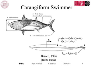
![Hydrodynamics
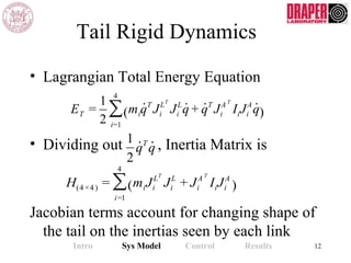
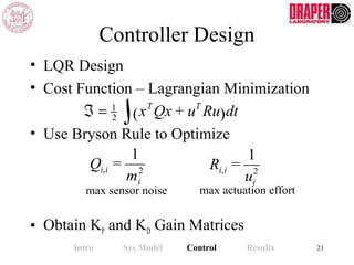
• Two Major Assumptions of EBT
1. Body Slope fore-aft is negligible [violated]
• Body slope is not extreme and EBT will slightly
overestimate added mass – acceptable engineering
approximation
1. Rigid Cylinder approx for added mass if the
undulation wavelength is at least 5 times the
section depth [good]
Intro Sys Model Control Results 14](https://image.slidesharecdn.com/vcuuv-160521145225/85/Fish-Propulsion-12-320.jpg)
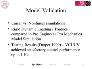

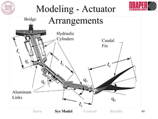
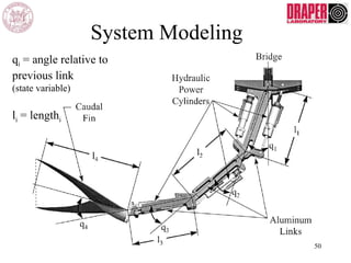
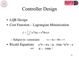
![System Modeling
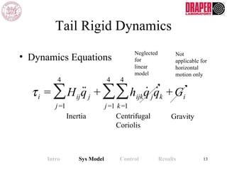
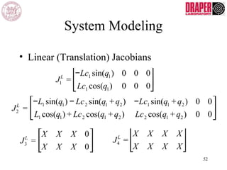
• Angular (Rotation) Jacobian
J1
A
= q1 0 0 0[ ]
J2
A
= q1 q2 0 0[ ]
J3
A
= q1 q2 q3 0[ ]
J4
A
= q1 q2 q3 q4[ ]
53](https://image.slidesharecdn.com/vcuuv-160521145225/85/Fish-Propulsion-48-320.jpg)
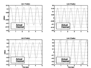
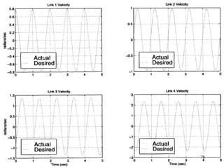
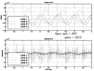
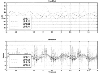

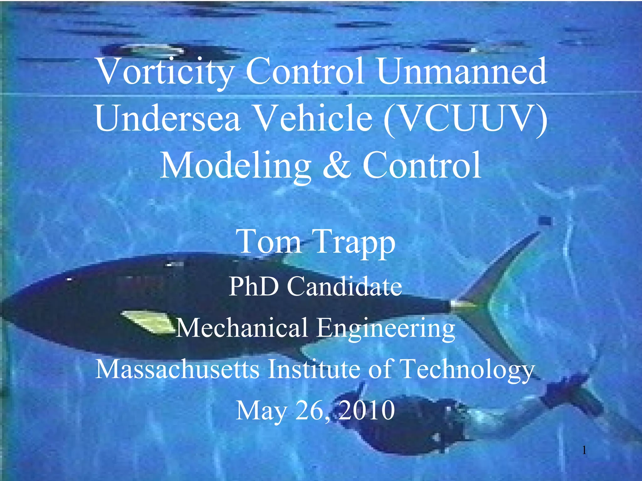
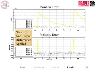
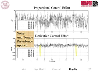
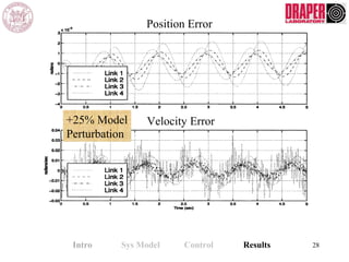
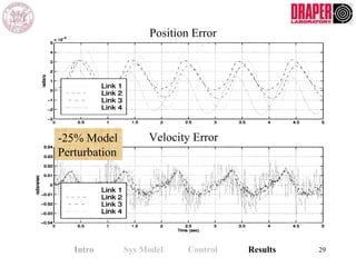
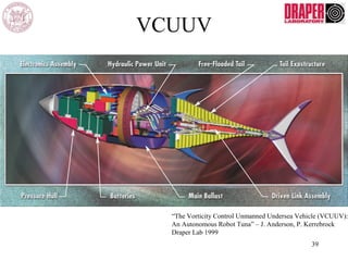
The document describes modeling and control of a Vorticity Control Unmanned Undersea Vehicle (VCUUV) being developed at MIT. It presents the nonlinear rigid body and hydrodynamic models of the vehicle's tail system, which consists of 4 hydraulically operated links that emulate fish swimming. A state-space controller is designed using computed torque and LQR approaches to control the tail's motion and reject disturbances. Simulation results show the controller effectively maintained position and velocity accuracy despite noise, disturbances, and model perturbations.


