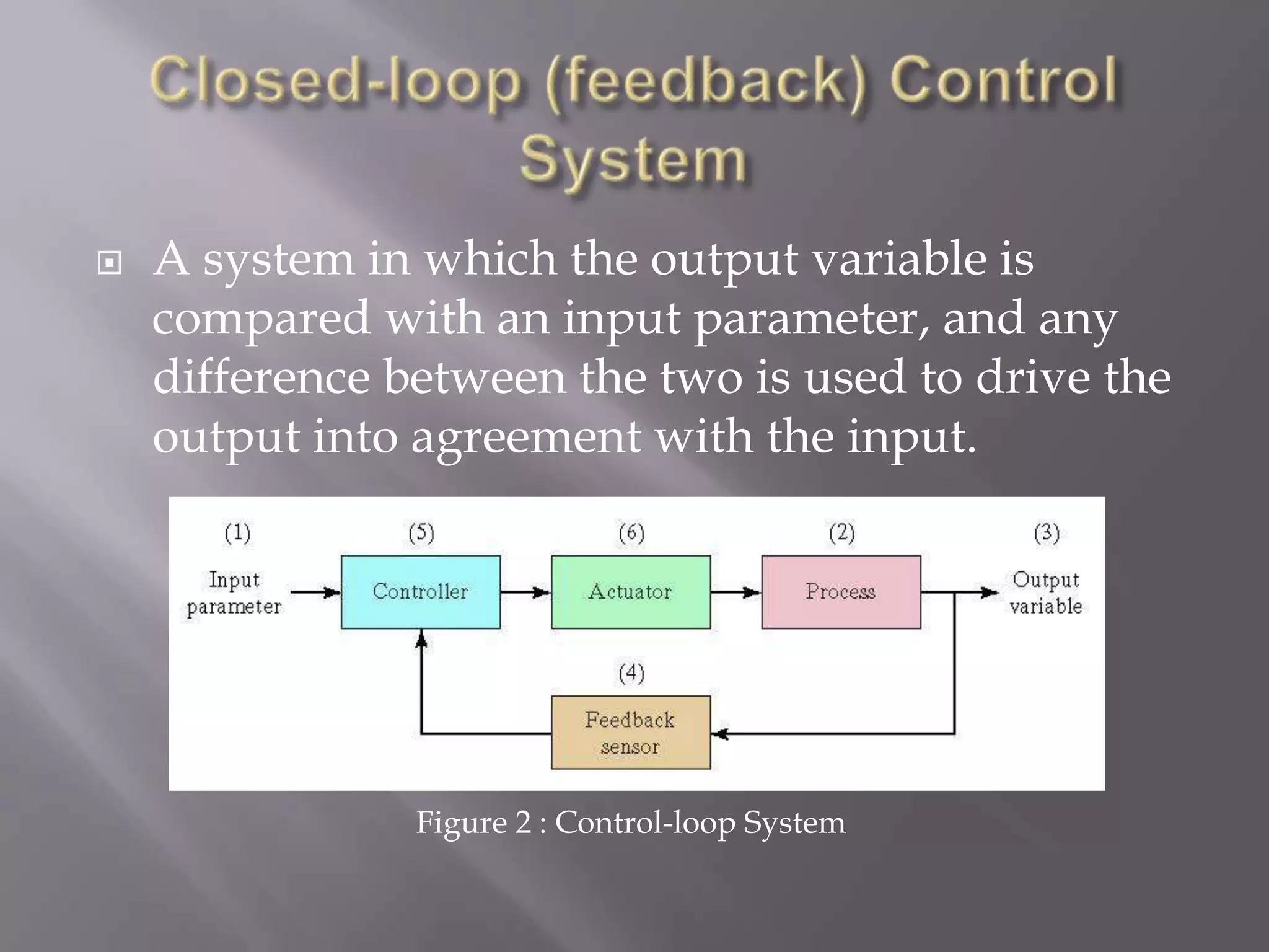
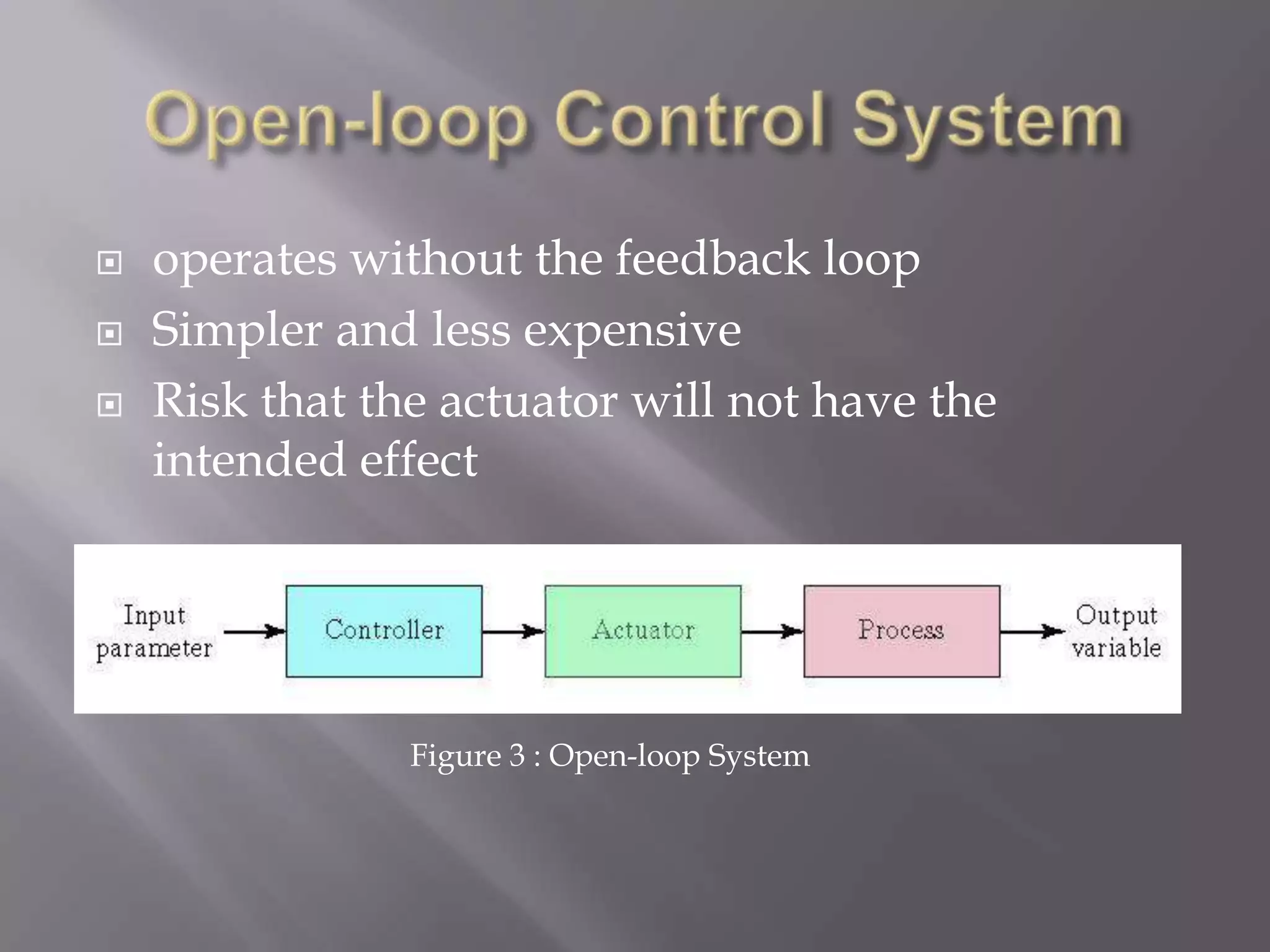
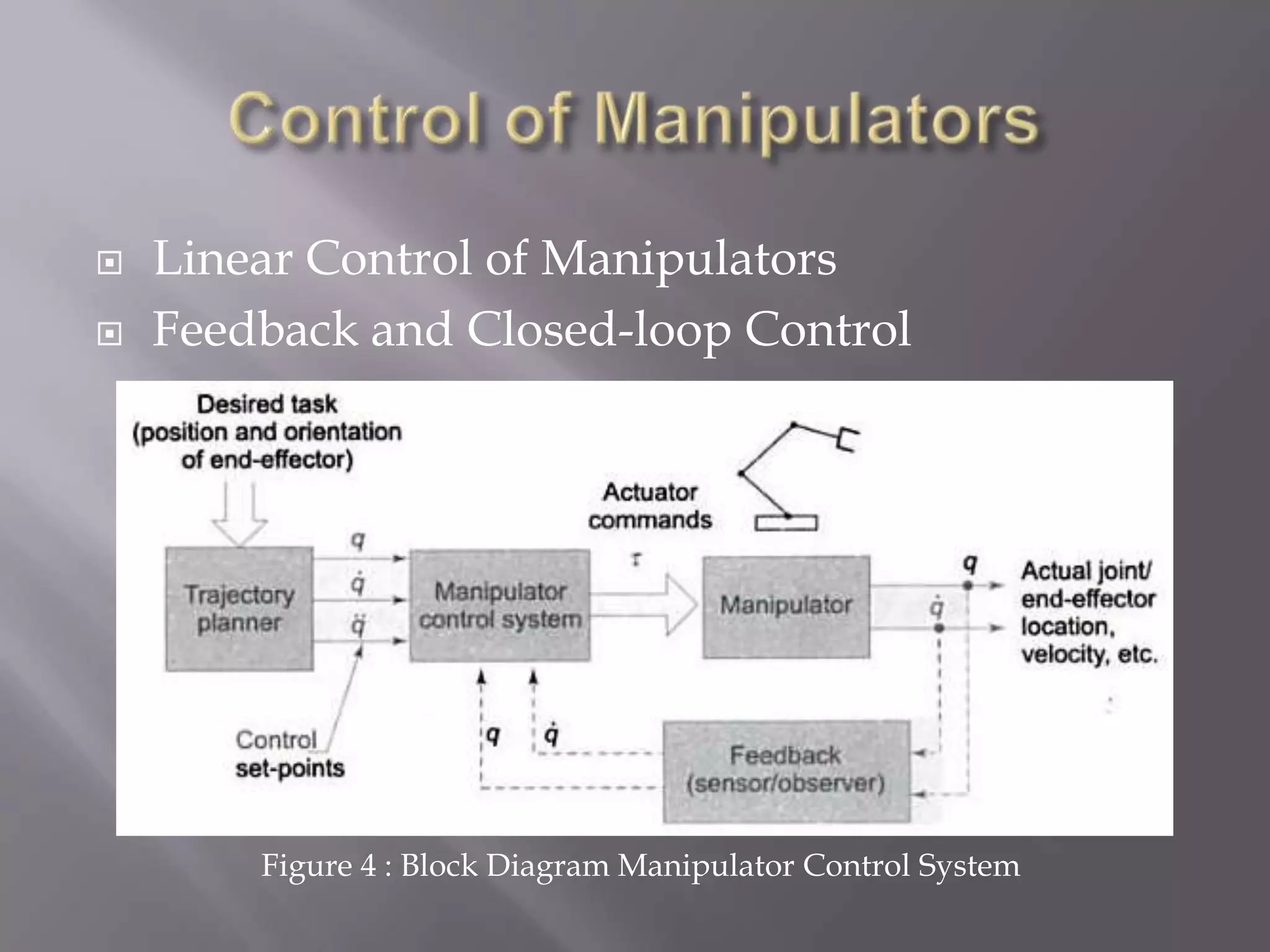
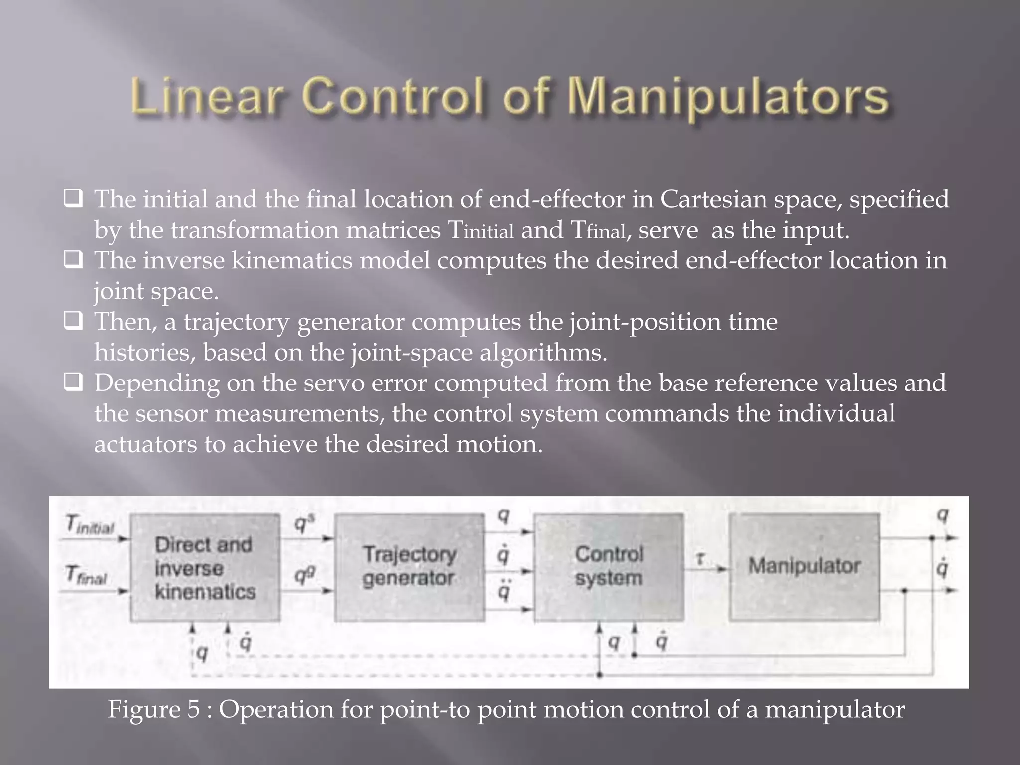
MOHAMMAD SYAZWAN BIN TALIB             B020910019
MUHAMAD HAFFIZ BIN MOHD RADZI          B020910190
MUHAMMAD SHAKIR BIN SULAIMAN           B020810095
MUHAMMAD FARHAN BIN MOHD ROSLAN        B020910115


           EN. RIDZA AZRI BIN RAMLEE


FAKULTI KEJURUTERAAN ELEKTRONIK & KEJURUTERAAN
                   KOMPUTER
   To learn open-loop and close loop system
   To learn linear and nonlinear control
   To design a simple manipulator controller
    based on several techniques
   Limited Sequence Control – pick-and-place
    operations using mechanical stops to set positions.
   Playback with point to point control – records
    work cycle as a sequence of points, then plays back
    the sequence during program execution.
   Playback with continuous path control – greater
    memory capacity and/or interpolation capability
    to execute paths (in addition to points).
   Intelligent control – exhibits behavior that makes it
    seem intelligent, e.g., responds to sensor
    inputs, makes decisions, communicates with
    humans.
   Electric
    – Uses electric motors to actuate individual joints
    – Preferred drive system in today's robots
   Hydraulic
    – Uses hydraulic pistons and rotary vane actuators
    – Noted for their high power and lift capacity
   Pneumatic
    – Typically limited to smaller robots and simple
    material transfer applications
Figure 1 : Hierarchical Control Structure
   Closed-loop (feedback) control system
   Open-loop control system
   A system in which the output variable is
    compared with an input parameter, and any
    difference between the two is used to drive the
    output into agreement with the input.


                Figure 2 : Control-loop System
   operates without the feedback loop
   Simpler and less expensive
   Risk that the actuator will not have the
    intended effect


                Figure 3 : Open-loop System
   Linear Control of Manipulators
   Feedback and Closed-loop Control


        Figure 4 : Block Diagram Manipulator Control System
 The initial and the final location of end-effector in Cartesian space, specified
  by the transformation matrices Tinitial and Tfinal, serve as the input.
 The inverse kinematics model computes the desired end-effector location in
  joint space.
 Then, a trajectory generator computes the joint-position time
  histories, based on the joint-space algorithms.
 Depending on the servo error computed from the base reference values and
  the sensor measurements, the control system commands the individual
  actuators to achieve the desired motion.


    Figure 5 : Operation for point-to point motion control of a manipulator
   The use of linear-control techniques is valid only when the
    system being studied can be modeled mathematically by
    linear differential equations.
   We have to calculate joint position time histories that
    correspond to desired end-effector motions through space.
   For the case of manipulator control, such linear methods
    must be viewed as approximate methods, for the dynamics
    of a manipulator are more properly represented by a
    nonlinear differential equation.
   It is often reasonable to make such approximations
    methods are most often used in current industrial practice.
   The justification for using linear controllers is not only
    empirical.
   There is a certain linear controller leads to a reasonable
    control system even without resorting to a linear
    approximation of manipulator dynamics.
   A control system that makes use of feedback is called a
    closed-loop control system. The "loop" closed by such
    a control system around the manipulator is apparent in
    the figure.
   The only way to build a high-performance control
    system is to make use of feedback from joint
    sensors, as indicated in the figure.
   Typically, this feedback is used to compute the servo
    error by finding the difference between the desired
    and the actual position and that between the desired
    and the actual velocity.
   The control system can then compute how much
    torque is required as a function to reduce servo errors.
   The central problem is designing a closed-loop system
    that meets certain performance specifications.
   First of all, the system has to remain stable. We will
    define a system to be stable, if the errors remain "small"
    when executing various desired trajectories even in the
    presence of some disturbances. An improperly designed
    control system can sometimes result in unstable
    performance, in which servo errors are enlarged instead
    of reduced.
   The second requirement is that the closed-loop
    performance of the system is satisfactory. In
    practice, such "proofs" range from mathematical proofs
    based on certain assumptions and models to more
    empirical results, such as those obtained through
    simulation or experimentation.
Figure 6 : Robot Control Architecture for n-DOF manipulator
   The manipulator control problem is a multi-
    input, multi-output (MIMO)problem, involving joint
    and the end-effector
    locations, velocities, accelerations, and force vectors.
   To simplify the problem, each joint is considered to be
    independent and separately controlled.
   This single-joint model is assumed to have a single
    input(set point) and single
    output(location, velocity, etc..).
   Hence, the n-DOF manipulator is modelled as n-
    independent linear second-order system and is
    controlled by n-independent single-input, single-
    output (SISO)control systems.
   Before developing and analyzing the linear second-
    order SISO model of the joint, the general second-order
    linear system characteristics are briefly brushed up
    first.
To overcome unmodeled dynamics, variable
payloads, fiction and disturbance torque, variation
and noise, we use nonlinear control to :
  Tracking, regulate state, state set point

  Ensure the desired stability properties

  Ensure the appropriate transients

  Reduce the sensitivity to plant parameters
A lot of techniques that are used for nonlinear
systems come from linear systems, because:
  Nonlinear systems can (sometime) be
   approximated by linear systems.
  Nonlinear systems can (sometime) be
   “transformed "into linear systems.
  The tools are generalized and extended.
Figure 5 : Flow Diagram Process
Figure 5 : Mechanical model of geared manipulators
   Transfer Function
   State Space
   Proportional and Derivative Control (PD)
   Proportional Integral and Derivatives (PID)
   State Space Controller (Poles Placement
    Technique)
   Artificial Intelligence Controller (Fuzzy Logic &
    Neural Network)
   Adaptive Cruise Controller (ACC)
   Cooperative Adaptive Cruise Controller (CACC)
   Model Predictive Controller (MPC).
   Robust Control and etc..
   John J. Craig - Introduction To Robotics -
    Mechanics And Control.
   R K Mittal & I J Nagrath, “Robotics and
    Control”, Tata McGraw-Hill Publishing
    Company. Ltd., New Delhi,2003
Chapter 8 - Robot Control System

Chapter 8 - Robot Control System

  • 1.
    MOHAMMAD SYAZWAN BINTALIB B020910019 MUHAMAD HAFFIZ BIN MOHD RADZI B020910190 MUHAMMAD SHAKIR BIN SULAIMAN B020810095 MUHAMMAD FARHAN BIN MOHD ROSLAN B020910115 EN. RIDZA AZRI BIN RAMLEE FAKULTI KEJURUTERAAN ELEKTRONIK & KEJURUTERAAN KOMPUTER
  • 2.
    To learn open-loop and close loop system  To learn linear and nonlinear control  To design a simple manipulator controller based on several techniques
  • 3.
    Limited Sequence Control – pick-and-place operations using mechanical stops to set positions.  Playback with point to point control – records work cycle as a sequence of points, then plays back the sequence during program execution.  Playback with continuous path control – greater memory capacity and/or interpolation capability to execute paths (in addition to points).  Intelligent control – exhibits behavior that makes it seem intelligent, e.g., responds to sensor inputs, makes decisions, communicates with humans.
  • 4.
    Electric – Uses electric motors to actuate individual joints – Preferred drive system in today's robots  Hydraulic – Uses hydraulic pistons and rotary vane actuators – Noted for their high power and lift capacity  Pneumatic – Typically limited to smaller robots and simple material transfer applications
  • 5.
    Figure 1 :Hierarchical Control Structure
  • 6.
    Closed-loop (feedback) control system  Open-loop control system
  • 7.
    A system in which the output variable is compared with an input parameter, and any difference between the two is used to drive the output into agreement with the input. Figure 2 : Control-loop System
  • 8.
    operates without the feedback loop  Simpler and less expensive  Risk that the actuator will not have the intended effect Figure 3 : Open-loop System
  • 9.
    Linear Control of Manipulators  Feedback and Closed-loop Control Figure 4 : Block Diagram Manipulator Control System
  • 10.
     The initialand the final location of end-effector in Cartesian space, specified by the transformation matrices Tinitial and Tfinal, serve as the input.  The inverse kinematics model computes the desired end-effector location in joint space.  Then, a trajectory generator computes the joint-position time histories, based on the joint-space algorithms.  Depending on the servo error computed from the base reference values and the sensor measurements, the control system commands the individual actuators to achieve the desired motion. Figure 5 : Operation for point-to point motion control of a manipulator
  • 11.
    The use of linear-control techniques is valid only when the system being studied can be modeled mathematically by linear differential equations.  We have to calculate joint position time histories that correspond to desired end-effector motions through space.  For the case of manipulator control, such linear methods must be viewed as approximate methods, for the dynamics of a manipulator are more properly represented by a nonlinear differential equation.  It is often reasonable to make such approximations methods are most often used in current industrial practice.  The justification for using linear controllers is not only empirical.  There is a certain linear controller leads to a reasonable control system even without resorting to a linear approximation of manipulator dynamics.
  • 12.
    A control system that makes use of feedback is called a closed-loop control system. The "loop" closed by such a control system around the manipulator is apparent in the figure.  The only way to build a high-performance control system is to make use of feedback from joint sensors, as indicated in the figure.  Typically, this feedback is used to compute the servo error by finding the difference between the desired and the actual position and that between the desired and the actual velocity.  The control system can then compute how much torque is required as a function to reduce servo errors.
  • 13.
    The central problem is designing a closed-loop system that meets certain performance specifications.  First of all, the system has to remain stable. We will define a system to be stable, if the errors remain "small" when executing various desired trajectories even in the presence of some disturbances. An improperly designed control system can sometimes result in unstable performance, in which servo errors are enlarged instead of reduced.  The second requirement is that the closed-loop performance of the system is satisfactory. In practice, such "proofs" range from mathematical proofs based on certain assumptions and models to more empirical results, such as those obtained through simulation or experimentation.
  • 14.
    Figure 6 :Robot Control Architecture for n-DOF manipulator
  • 15.
    The manipulator control problem is a multi- input, multi-output (MIMO)problem, involving joint and the end-effector locations, velocities, accelerations, and force vectors.  To simplify the problem, each joint is considered to be independent and separately controlled.  This single-joint model is assumed to have a single input(set point) and single output(location, velocity, etc..).  Hence, the n-DOF manipulator is modelled as n- independent linear second-order system and is controlled by n-independent single-input, single- output (SISO)control systems.  Before developing and analyzing the linear second- order SISO model of the joint, the general second-order linear system characteristics are briefly brushed up first.
  • 16.
    To overcome unmodeleddynamics, variable payloads, fiction and disturbance torque, variation and noise, we use nonlinear control to :  Tracking, regulate state, state set point  Ensure the desired stability properties  Ensure the appropriate transients  Reduce the sensitivity to plant parameters
  • 17.
    A lot oftechniques that are used for nonlinear systems come from linear systems, because:  Nonlinear systems can (sometime) be approximated by linear systems.  Nonlinear systems can (sometime) be “transformed "into linear systems.  The tools are generalized and extended.
  • 18.
    Figure 5 :Flow Diagram Process
  • 19.
    Figure 5 :Mechanical model of geared manipulators
  • 20.
    Transfer Function  State Space
  • 21.
    Proportional and Derivative Control (PD)  Proportional Integral and Derivatives (PID)  State Space Controller (Poles Placement Technique)  Artificial Intelligence Controller (Fuzzy Logic & Neural Network)  Adaptive Cruise Controller (ACC)  Cooperative Adaptive Cruise Controller (CACC)  Model Predictive Controller (MPC).  Robust Control and etc..
  • 22.
    John J. Craig - Introduction To Robotics - Mechanics And Control.  R K Mittal & I J Nagrath, “Robotics and Control”, Tata McGraw-Hill Publishing Company. Ltd., New Delhi,2003