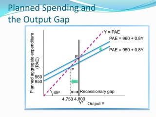
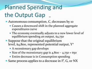
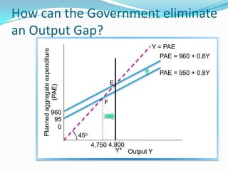
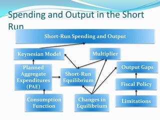
This document provides an overview of key concepts in the basic Keynesian macroeconomic model. It defines planned aggregate expenditure and its components. It then explains how the economy reaches short-run equilibrium where planned spending equals output. It demonstrates how a change in an autonomous spending component, like consumption, can cause the equilibrium to change and create an output gap. The income-expenditure multiplier is introduced to show how a $1 change in spending can impact output. Finally, it discusses how fiscal policy tools like government spending or tax changes can be used to address output gaps according to the Keynesian model.


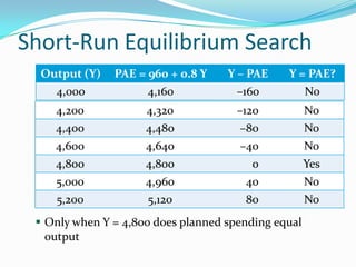
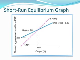
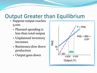
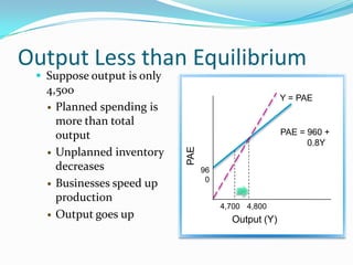


![Tahreem_Kousar_EconomicsSSSSSSSS_file[1].pptx](https://cdn.slidesharecdn.com/ss_thumbnails/tahreemkousareconomicsfile1-250617080609-d0ff08be-thumbnail.jpg?width=640&height=640&fit=bounds)


