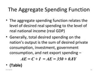
Determination of GDP in the
Short Term
Lecture 3
Outline
• Macroeconomic theory explains the deviation of
actual from potential GDP (i.e. GDP gap)
• Determination of GDP in the short run depends
on the behaviour of key categories of (C, I, G, NX)
• Consumption spending depends on disposable
income and wealth
• Investment spending depends on real interest
rates and business confidence
• A necessary condition for GDP to be in
equilibrium is that desired domestic spending is
equal to actual output
207/14/14
• The central problem for macroeconomic
policy-makers is to decide how to manage the
economy in such a way that inflation is kept
under control while unemployment is also
kept to a minimum
• Virtually all economies have some periods
when actual GDP is growing faster than
potential and other periods when it is growing
more slowly than potential, or even falling
• In other words, actual economies exhibit
cycles about the trend growth path
307/14/14
• Periods of decline in actual GDP (or even
when growth in actual GDP is below potential)
are costly because they are associated with a
loss of output that is gone forever
• Economic downturns do not typically lead to
all citizens loosing some equal amount of
income – rather, they lead to some people
losing their jobs (or businesses) and thereby
suffering loss of income and well-being
407/14/14
• Unemployment is undesirable, and is
commonly agreed that policy-makers should
aim to sustain unemployment a low level
• The outcome of an excessive growth in
demand relative to supply is inflation, which is
disruptive to the economy
5
SO
07/14/14
Key Assumptions on Macro Theory
• Aggregation across industries
– In elementary macro economics, we assume the existence
of a single productive sector producing a homogeneous
output
• Time-scale
– Short run- the period during which the economy maintains
a deviation of actual from potential output, or a GDP gap.
This deviation is associated with the existence of excess
capacity and unemployment (recession), or with
unsustainable output and inflation (boom)
– Analysis of the short run in macroeconomics is concerned
with explaining why national output can deviate from its
potential level. It is about the GDP gap and how to keep
both positive and negative gaps as small as possible
– That is, how do we keep actual GDP as close as possible to
potential GDP?
607/14/14
Key Assumptions on Macro Theory
• Long run- a period sufficient to allow time for
the automatic adjustment mechanisms to
return economic activity to equilibrium after
it has been disturbed by an exogenous shock
– This equilibrium is reached when the economy
returns to producing the level of potential (or full
employment) output
– We assume that the long run level of output is
constant and is associated with a fixed capital
stock and a fixed level of technical knowledge
707/14/14
Temporary Assumptions
• The price level
– We assume that the price level (the money price of the
economy’s single output good) is fixed
– Hence all variables must necessarily be measured in real
terms
• Excess capacity
– We assume the economy has excess capacity so that is not
constrained from producing more output by shortages of
capital stock or labour
• Closed economy
– We ignore the possibility that the output of the economy
can be sold overseas and that domestic consumers can
buy foreign-produced goods
• No government
807/14/14
Summarising Assumptions
• We have a closed economy with a single
industrial sector, producing a homogeneous
output, at a fixed price, with no government.
There is also excess capacity, so there are no
resource constraints preventing the expansion
of national output
907/14/14
What Determines Aggregate
Spending
From actual to desired spending
• Desired (planned/intended) spending – refers to what
people want to spend out of the resources that are at their
command
– Desired private consumption, desired investment, desired
government consumption, and desired exports (total desired
spending on domestically produced goods and services, called
aggregate spending, or AE = C + I + G + (X – IM))
• The National Accounts measure actual spending in each of
the four categories: private consumption, investment,
government consumption, and net exports. The theory of
GDP determination deals with desired spending in each of
these four categories
1007/14/14
What Determines Aggregate
Spending II
Autonomous and Induced Spending
• Autonomous (exogenous) spending –
components of aggregate spending that do
not depend on current domestic incomes
– Autonomous spending can and does change, but
such changes do not occur systematically in
response to changes in income)
• Induced (or endogenous) spending –
components of aggregate spending that do
change in response to changes in income
1107/14/14
What Determines Aggregate
Spending III
Desired private consumption spending
• There are only two possible uses of disposable
income: consumption and saving. So when each
individual decides how much to put to one use,
she has automatically decided how much to put
to the other use
• What determines the division between the
amount that people decide to spend on goods
and services for consumption and the amount
that they decide to save?
– Consumption function and saving function
1207/14/14
• Consumption function relates the total desired consumer
spending of the personal sector to the variables that affect it
• Under the assumptions, there are no taxes
– Individuals receive all income that is generated
– Therefore, disposable income Yd is equal to national income, Y
• The term consumption function describes the relationship
between private consumption and the variables that
influence it. In the simplest theory, consumption spending is
determined by current disposable income
– When income is zero, a typical individual will still (via borrowing,
or drawing down savings) consume some minimal amount (i.e.
autonomous)
– The higher a person’s income, the more he or she will want to
consume (i.e. induced). Table
1307/14/14
The slope of the consumption function
• Properties of the short-term consumption
function as follows
– There is a break-even level of income at which
APC equals unity.
– Below this level APC is greater than unity; above
it APC is less than unity.
– Below the break-even level consumption exceeds
income, so consumers run down savings or
borrow.
– Above the break-even level income exceeds
consumption, so there is positive saving
1407/14/14
The slope of the consumption function
• Properties of the short-term consumption
function as follows
– MPC is greater than zero, but less than unity, for
all levels of income.
– This means that for each additional GHȼ1 of
income, less than GHȼ1 is spent on consumption
and the rest saved.
– For a straight-line consumption function, the MPC
is constant at all levels of income
1507/14/14
The saving function
• Once we know the dependence of consumption on
disposable income, we also automatically know the
dependence of saving on disposable income
• We also have APS and MPS
• There is a simple relationship between the saving and
consumption propensities
• APC and APS must sum to unity (1), just like MPC and
MPS
• Because income is either spent or saved, it follows that
the fractions of incomes consumed and saved must
account for all income (APC + APS = 1)
• It also follows that the fractions of any increment to
income consumed and saved must account for all of
that increment (MPC + MPS = 1)
1607/14/14
• What happens when there is an unexpected rise in
wealth?
– Less of current disposable income needs to be saved for
the future
– Will tend to cause a larger fraction of disposable income to
be spent on consumption and a smaller fraction to be
saved
– This will shift the consumption function upward and saving
function downward
• A fall in wealth
– Increases the incentive to save in order to restore wealth
– This shifts the consumption function downward and saving
function upward
• What about interest rate and consumer spending?
1707/14/14
Desired investment Spending
• Investment spending is the most volatile
component of GDP and
• Changes in investment spending are strongly
associated with economic fluctuations
• What is the relationship between Investment and
the Real interest rate
• Other things being equal, the higher the real
interest rate, the higher is the cost of borrowing
money for investment purposes and the less is
the amount of desired investment spending
1807/14/14
• Inventory accumulation
– The higher the real rate of interest, the lower is the
desired inventory of goods and materials. Changes in
the rate of interest cause temporary bouts of
investments (or disinvestment) as inventories are
either increased or decreased
• Residential housing construction
– Spending for residential construction tends to vary
negatively with interest rates
• Business fixed capital formation
– Increase in real interest rates means that the
opportunity cost of investing in fixed capital had risen
1907/14/14
• Expectations and business confidence
– Business investments depends in part on firms’
forecasts of the future state of the economy
– When firms expect good times ahead they will
want to invest so as to reap future profits
– When they expect bad times they will not invest,
because, given their expectations, there will be no
payoff from doing so
2007/14/14
The Aggregate Spending Function
• The aggregate spending function relates the
level of desired real spending to the level of
real national income (real GDP)
• Generally, total desired spending on the
nation’s output is the sum of desired private
consumption, investment, government
consumption, and net export spending –
AE = C + I = AE = 350 + 0.8Y
• (Table)
2107/14/14
The propensity to spend out of national income
• Marginal propensity to spend (c) – the fraction
of any increment to national income (GDP) that
will be spent on purchasing domestic output
(∆AE/∆Y)
– The slope of the AE function
• Marginal propensity not to spend (1 – c) – the
fraction of an increment to national income that
does not add to desired aggregate spending
• Note – know the difference between the MPC
and MPS and MPnS and MPS
2207/14/14
Equilibrium GDP
• When something is in equilibrium there is no
tendency for it to change, forces are acting on it,
but they balance out, and the net result is no
change
– At any level of GDP at which aggregate desired
spending exceeds total output, there will be pressure
for GDP to rise caused by:
• Queues and unfulfilled order books
• Extra sales after reduction in inventories
– At any level of GDP for which aggregate desired
spending is less than total output, there will be
pressure for GDP to fall
– The equilibrium level of GDP occurs where aggregate
desired spending equals total output
2307/14/14
Changes in GDP
Suppose desired aggregate spending rises
• This may be as a response to a change in GDP
(incomes) – movement along the AE function,
or
• It may be the result of an increased desire to
spend at each level of GDP – shift in the AE
function
2407/14/14
Shifts in the Aggregate Spending Function
• Upward Shifts
– If individuals permanently increase their levels of
desired consumption spending at each level of
disposable income
– A major company desires to invest in more fixed
capital
• Two types of upward shift
– If the same addition to spending occurs at all levels of
income the AE line shifts parallel to itself
– If there is a change in the propensity to spend out of
national income, the slope of the AE line changes
2507/14/14
• Downward shifts
– Decrease in the amount of consumption at each level of
income
– Decrease in the amount of investment spending at each
level of income
• 2 General Propositions of the theory of GDP
determination
– A rise in the amount of desired aggregate spending that
is associated with each level of national income will
increase equilibrium national output (GDP)
– A fall in the amount of desired aggregate spending that
is associated with each level of national income will
lower equilibrium national output (GDP)
2607/14/14
The Multiplier
• We know how to predict the direction of changes in
GDP that will occur in response to various shifts in the
aggregate spending function
• How can we predict the magnitude of these changes?
• The multiplier is the measure of the magnitude of
changes in GDP induced by a given change in
autonomous expenditure
• The ratio of the change in GDP to the change in
autonomous spending
• The simple multiplier measures the change in
equilibrium GDP that occurs in response to a change in
autonomous spending at a constant price level
• Why is the multiplier greater than 1
2707/14/14
The size of the Multiplier
• The larger the marginal propensity to spend,
the steeper is the aggregate spending function
and the larger is the multiplier
K = ∆Y/∆A = 1/1 – c
• The simple multiplier equals the reciprocal of
the marginal propensity not to spend
2807/14/14
Assignment
• Calculate GDP using the following information
(where there is no government and no foreign
trade): C = 100 + 0.8Y; I = 1,000.
2907/14/14

Lecture 3

  • 1.
    Determination of GDPin the Short Term Lecture 3
  • 2.
    Outline • Macroeconomic theoryexplains the deviation of actual from potential GDP (i.e. GDP gap) • Determination of GDP in the short run depends on the behaviour of key categories of (C, I, G, NX) • Consumption spending depends on disposable income and wealth • Investment spending depends on real interest rates and business confidence • A necessary condition for GDP to be in equilibrium is that desired domestic spending is equal to actual output 207/14/14
  • 3.
    • The centralproblem for macroeconomic policy-makers is to decide how to manage the economy in such a way that inflation is kept under control while unemployment is also kept to a minimum • Virtually all economies have some periods when actual GDP is growing faster than potential and other periods when it is growing more slowly than potential, or even falling • In other words, actual economies exhibit cycles about the trend growth path 307/14/14
  • 4.
    • Periods ofdecline in actual GDP (or even when growth in actual GDP is below potential) are costly because they are associated with a loss of output that is gone forever • Economic downturns do not typically lead to all citizens loosing some equal amount of income – rather, they lead to some people losing their jobs (or businesses) and thereby suffering loss of income and well-being 407/14/14
  • 5.
    • Unemployment isundesirable, and is commonly agreed that policy-makers should aim to sustain unemployment a low level • The outcome of an excessive growth in demand relative to supply is inflation, which is disruptive to the economy 5 SO 07/14/14
  • 6.
    Key Assumptions onMacro Theory • Aggregation across industries – In elementary macro economics, we assume the existence of a single productive sector producing a homogeneous output • Time-scale – Short run- the period during which the economy maintains a deviation of actual from potential output, or a GDP gap. This deviation is associated with the existence of excess capacity and unemployment (recession), or with unsustainable output and inflation (boom) – Analysis of the short run in macroeconomics is concerned with explaining why national output can deviate from its potential level. It is about the GDP gap and how to keep both positive and negative gaps as small as possible – That is, how do we keep actual GDP as close as possible to potential GDP? 607/14/14
  • 7.
    Key Assumptions onMacro Theory • Long run- a period sufficient to allow time for the automatic adjustment mechanisms to return economic activity to equilibrium after it has been disturbed by an exogenous shock – This equilibrium is reached when the economy returns to producing the level of potential (or full employment) output – We assume that the long run level of output is constant and is associated with a fixed capital stock and a fixed level of technical knowledge 707/14/14
  • 8.
    Temporary Assumptions • Theprice level – We assume that the price level (the money price of the economy’s single output good) is fixed – Hence all variables must necessarily be measured in real terms • Excess capacity – We assume the economy has excess capacity so that is not constrained from producing more output by shortages of capital stock or labour • Closed economy – We ignore the possibility that the output of the economy can be sold overseas and that domestic consumers can buy foreign-produced goods • No government 807/14/14
  • 9.
    Summarising Assumptions • Wehave a closed economy with a single industrial sector, producing a homogeneous output, at a fixed price, with no government. There is also excess capacity, so there are no resource constraints preventing the expansion of national output 907/14/14
  • 10.
    What Determines Aggregate Spending Fromactual to desired spending • Desired (planned/intended) spending – refers to what people want to spend out of the resources that are at their command – Desired private consumption, desired investment, desired government consumption, and desired exports (total desired spending on domestically produced goods and services, called aggregate spending, or AE = C + I + G + (X – IM)) • The National Accounts measure actual spending in each of the four categories: private consumption, investment, government consumption, and net exports. The theory of GDP determination deals with desired spending in each of these four categories 1007/14/14
  • 11.
    What Determines Aggregate SpendingII Autonomous and Induced Spending • Autonomous (exogenous) spending – components of aggregate spending that do not depend on current domestic incomes – Autonomous spending can and does change, but such changes do not occur systematically in response to changes in income) • Induced (or endogenous) spending – components of aggregate spending that do change in response to changes in income 1107/14/14
  • 12.
    What Determines Aggregate SpendingIII Desired private consumption spending • There are only two possible uses of disposable income: consumption and saving. So when each individual decides how much to put to one use, she has automatically decided how much to put to the other use • What determines the division between the amount that people decide to spend on goods and services for consumption and the amount that they decide to save? – Consumption function and saving function 1207/14/14
  • 13.
    • Consumption functionrelates the total desired consumer spending of the personal sector to the variables that affect it • Under the assumptions, there are no taxes – Individuals receive all income that is generated – Therefore, disposable income Yd is equal to national income, Y • The term consumption function describes the relationship between private consumption and the variables that influence it. In the simplest theory, consumption spending is determined by current disposable income – When income is zero, a typical individual will still (via borrowing, or drawing down savings) consume some minimal amount (i.e. autonomous) – The higher a person’s income, the more he or she will want to consume (i.e. induced). Table 1307/14/14
  • 14.
    The slope ofthe consumption function • Properties of the short-term consumption function as follows – There is a break-even level of income at which APC equals unity. – Below this level APC is greater than unity; above it APC is less than unity. – Below the break-even level consumption exceeds income, so consumers run down savings or borrow. – Above the break-even level income exceeds consumption, so there is positive saving 1407/14/14
  • 15.
    The slope ofthe consumption function • Properties of the short-term consumption function as follows – MPC is greater than zero, but less than unity, for all levels of income. – This means that for each additional GHȼ1 of income, less than GHȼ1 is spent on consumption and the rest saved. – For a straight-line consumption function, the MPC is constant at all levels of income 1507/14/14
  • 16.
    The saving function •Once we know the dependence of consumption on disposable income, we also automatically know the dependence of saving on disposable income • We also have APS and MPS • There is a simple relationship between the saving and consumption propensities • APC and APS must sum to unity (1), just like MPC and MPS • Because income is either spent or saved, it follows that the fractions of incomes consumed and saved must account for all income (APC + APS = 1) • It also follows that the fractions of any increment to income consumed and saved must account for all of that increment (MPC + MPS = 1) 1607/14/14
  • 17.
    • What happenswhen there is an unexpected rise in wealth? – Less of current disposable income needs to be saved for the future – Will tend to cause a larger fraction of disposable income to be spent on consumption and a smaller fraction to be saved – This will shift the consumption function upward and saving function downward • A fall in wealth – Increases the incentive to save in order to restore wealth – This shifts the consumption function downward and saving function upward • What about interest rate and consumer spending? 1707/14/14
  • 18.
    Desired investment Spending •Investment spending is the most volatile component of GDP and • Changes in investment spending are strongly associated with economic fluctuations • What is the relationship between Investment and the Real interest rate • Other things being equal, the higher the real interest rate, the higher is the cost of borrowing money for investment purposes and the less is the amount of desired investment spending 1807/14/14
  • 19.
    • Inventory accumulation –The higher the real rate of interest, the lower is the desired inventory of goods and materials. Changes in the rate of interest cause temporary bouts of investments (or disinvestment) as inventories are either increased or decreased • Residential housing construction – Spending for residential construction tends to vary negatively with interest rates • Business fixed capital formation – Increase in real interest rates means that the opportunity cost of investing in fixed capital had risen 1907/14/14
  • 20.
    • Expectations andbusiness confidence – Business investments depends in part on firms’ forecasts of the future state of the economy – When firms expect good times ahead they will want to invest so as to reap future profits – When they expect bad times they will not invest, because, given their expectations, there will be no payoff from doing so 2007/14/14
  • 21.
    The Aggregate SpendingFunction • The aggregate spending function relates the level of desired real spending to the level of real national income (real GDP) • Generally, total desired spending on the nation’s output is the sum of desired private consumption, investment, government consumption, and net export spending – AE = C + I = AE = 350 + 0.8Y • (Table) 2107/14/14
  • 22.
    The propensity tospend out of national income • Marginal propensity to spend (c) – the fraction of any increment to national income (GDP) that will be spent on purchasing domestic output (∆AE/∆Y) – The slope of the AE function • Marginal propensity not to spend (1 – c) – the fraction of an increment to national income that does not add to desired aggregate spending • Note – know the difference between the MPC and MPS and MPnS and MPS 2207/14/14
  • 23.
    Equilibrium GDP • Whensomething is in equilibrium there is no tendency for it to change, forces are acting on it, but they balance out, and the net result is no change – At any level of GDP at which aggregate desired spending exceeds total output, there will be pressure for GDP to rise caused by: • Queues and unfulfilled order books • Extra sales after reduction in inventories – At any level of GDP for which aggregate desired spending is less than total output, there will be pressure for GDP to fall – The equilibrium level of GDP occurs where aggregate desired spending equals total output 2307/14/14
  • 24.
    Changes in GDP Supposedesired aggregate spending rises • This may be as a response to a change in GDP (incomes) – movement along the AE function, or • It may be the result of an increased desire to spend at each level of GDP – shift in the AE function 2407/14/14
  • 25.
    Shifts in theAggregate Spending Function • Upward Shifts – If individuals permanently increase their levels of desired consumption spending at each level of disposable income – A major company desires to invest in more fixed capital • Two types of upward shift – If the same addition to spending occurs at all levels of income the AE line shifts parallel to itself – If there is a change in the propensity to spend out of national income, the slope of the AE line changes 2507/14/14
  • 26.
    • Downward shifts –Decrease in the amount of consumption at each level of income – Decrease in the amount of investment spending at each level of income • 2 General Propositions of the theory of GDP determination – A rise in the amount of desired aggregate spending that is associated with each level of national income will increase equilibrium national output (GDP) – A fall in the amount of desired aggregate spending that is associated with each level of national income will lower equilibrium national output (GDP) 2607/14/14
  • 27.
    The Multiplier • Weknow how to predict the direction of changes in GDP that will occur in response to various shifts in the aggregate spending function • How can we predict the magnitude of these changes? • The multiplier is the measure of the magnitude of changes in GDP induced by a given change in autonomous expenditure • The ratio of the change in GDP to the change in autonomous spending • The simple multiplier measures the change in equilibrium GDP that occurs in response to a change in autonomous spending at a constant price level • Why is the multiplier greater than 1 2707/14/14
  • 28.
    The size ofthe Multiplier • The larger the marginal propensity to spend, the steeper is the aggregate spending function and the larger is the multiplier K = ∆Y/∆A = 1/1 – c • The simple multiplier equals the reciprocal of the marginal propensity not to spend 2807/14/14
  • 29.
    Assignment • Calculate GDPusing the following information (where there is no government and no foreign trade): C = 100 + 0.8Y; I = 1,000. 2907/14/14