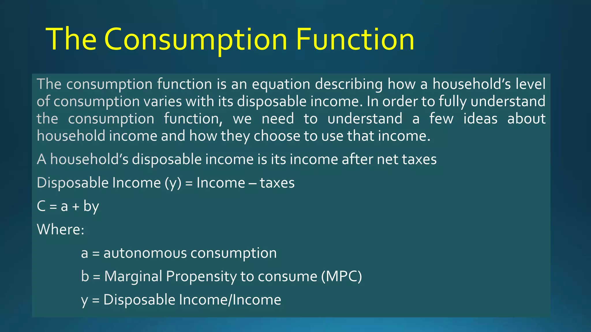
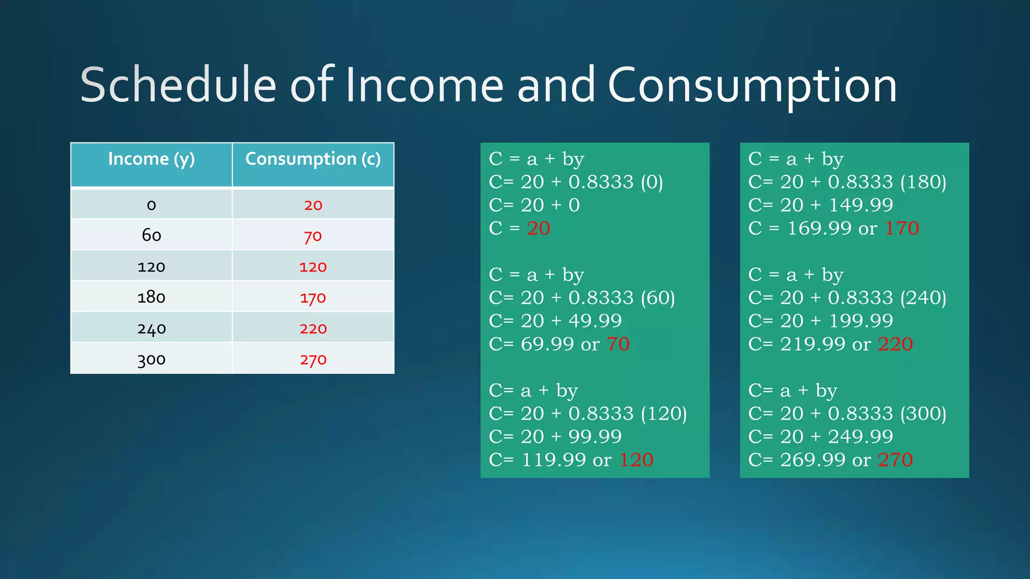
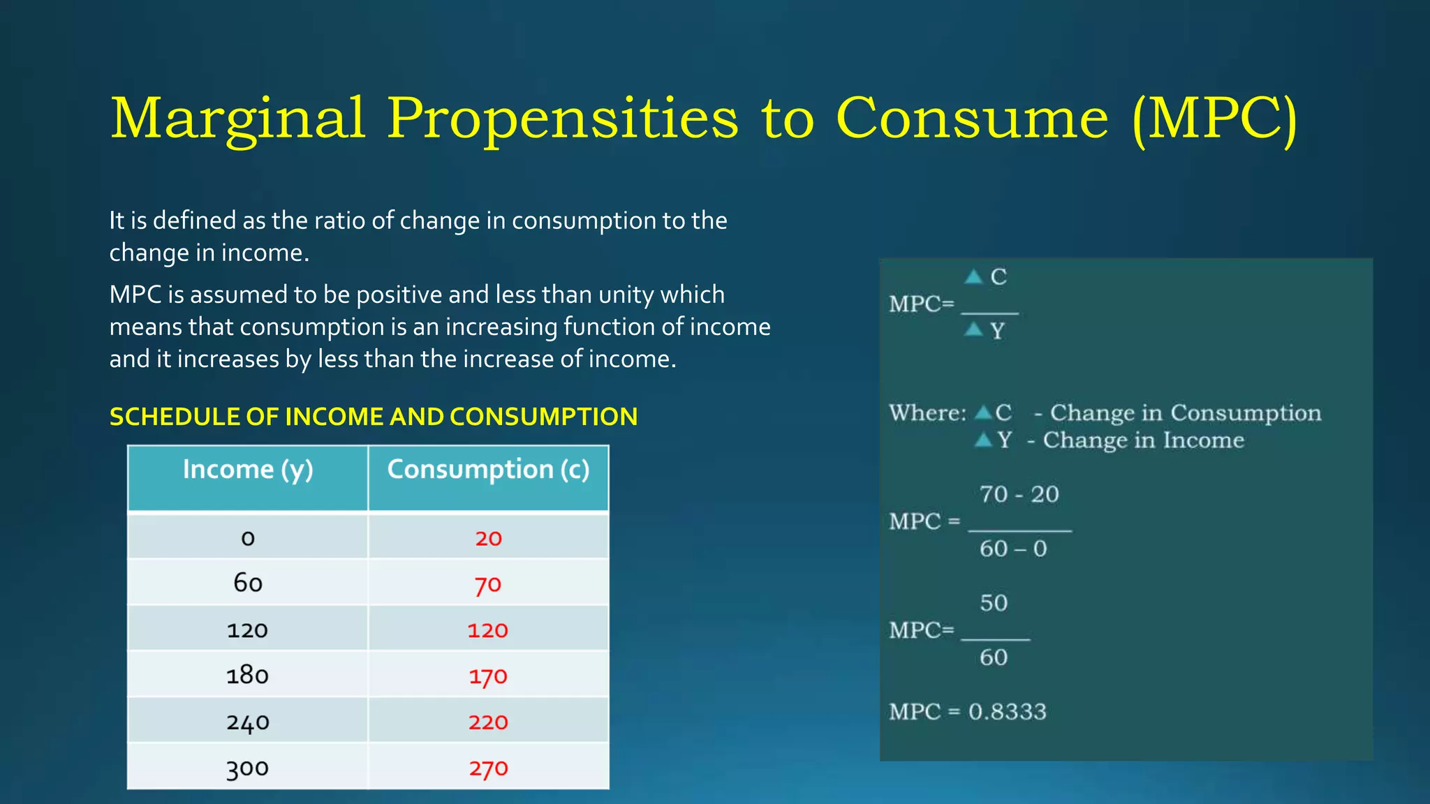
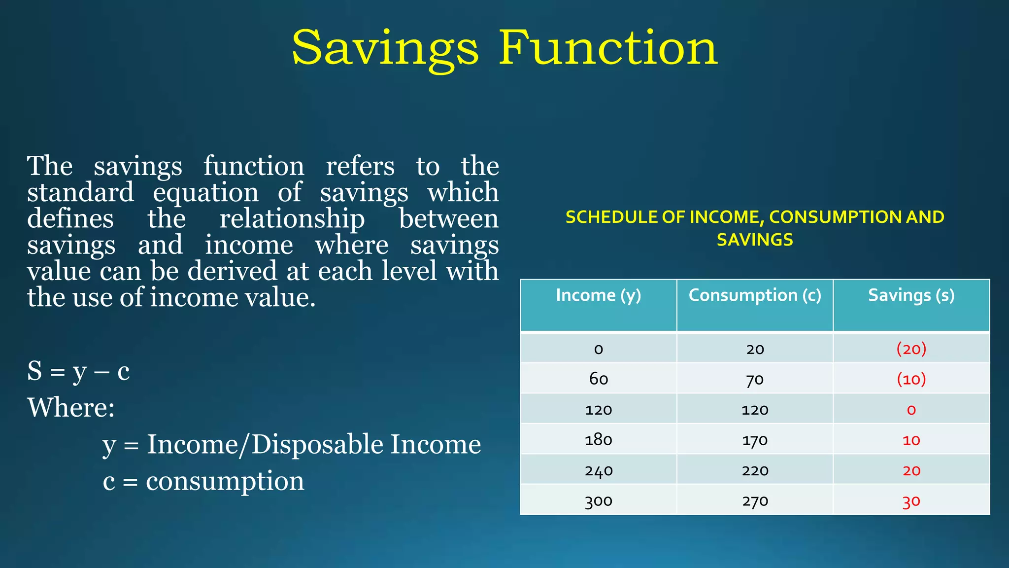
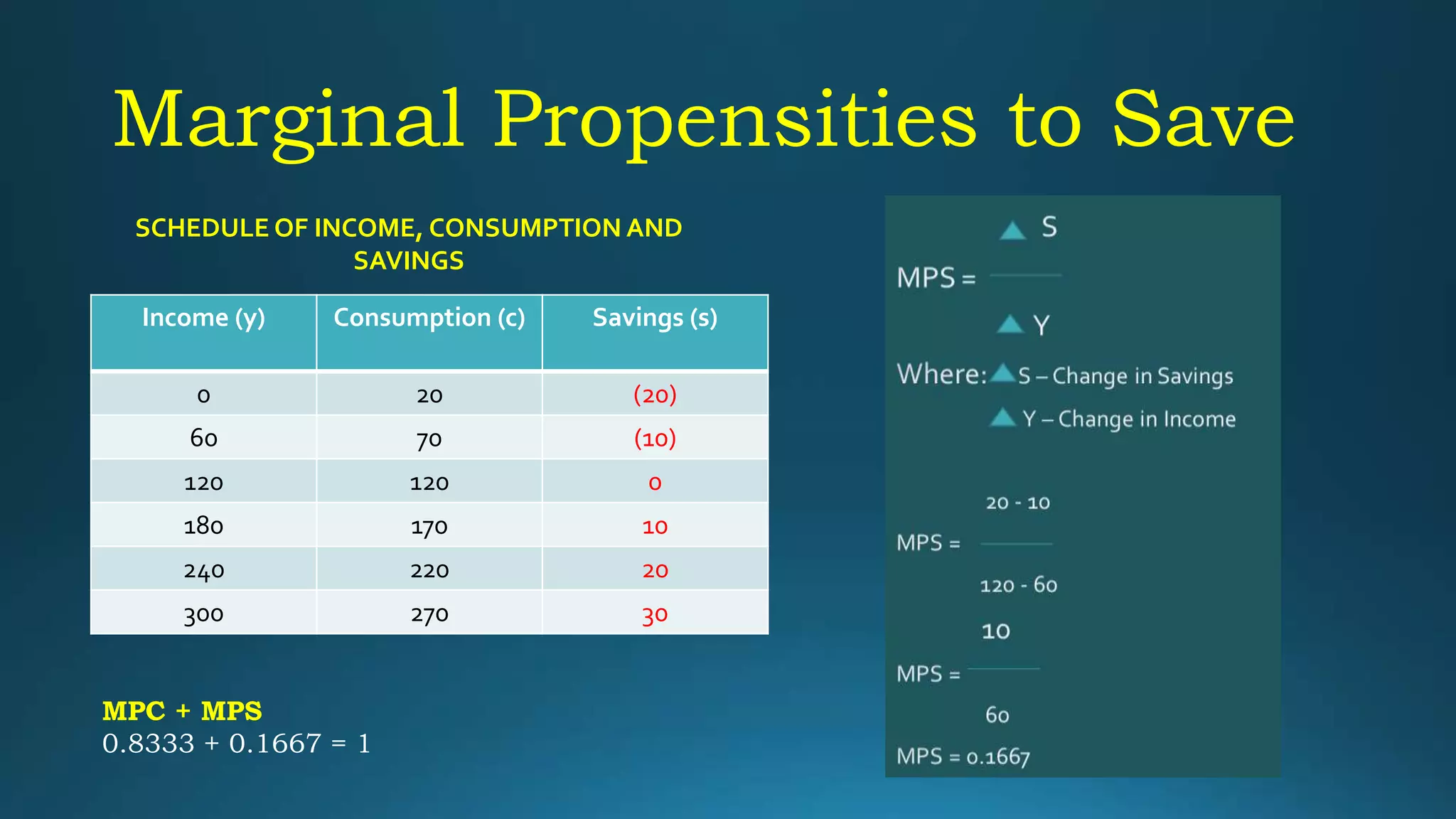
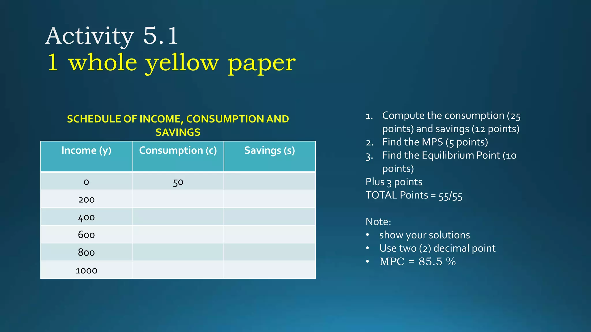
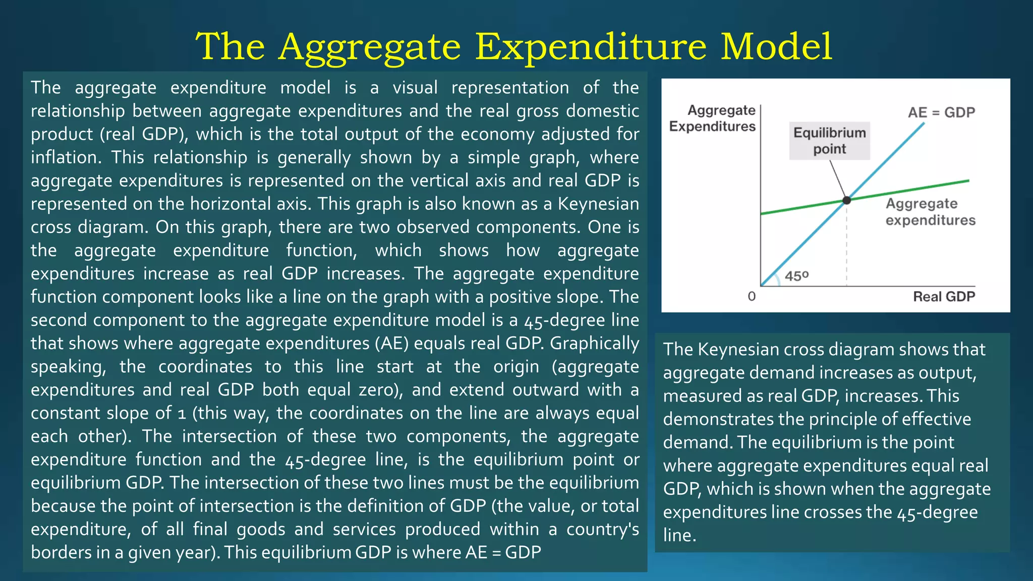
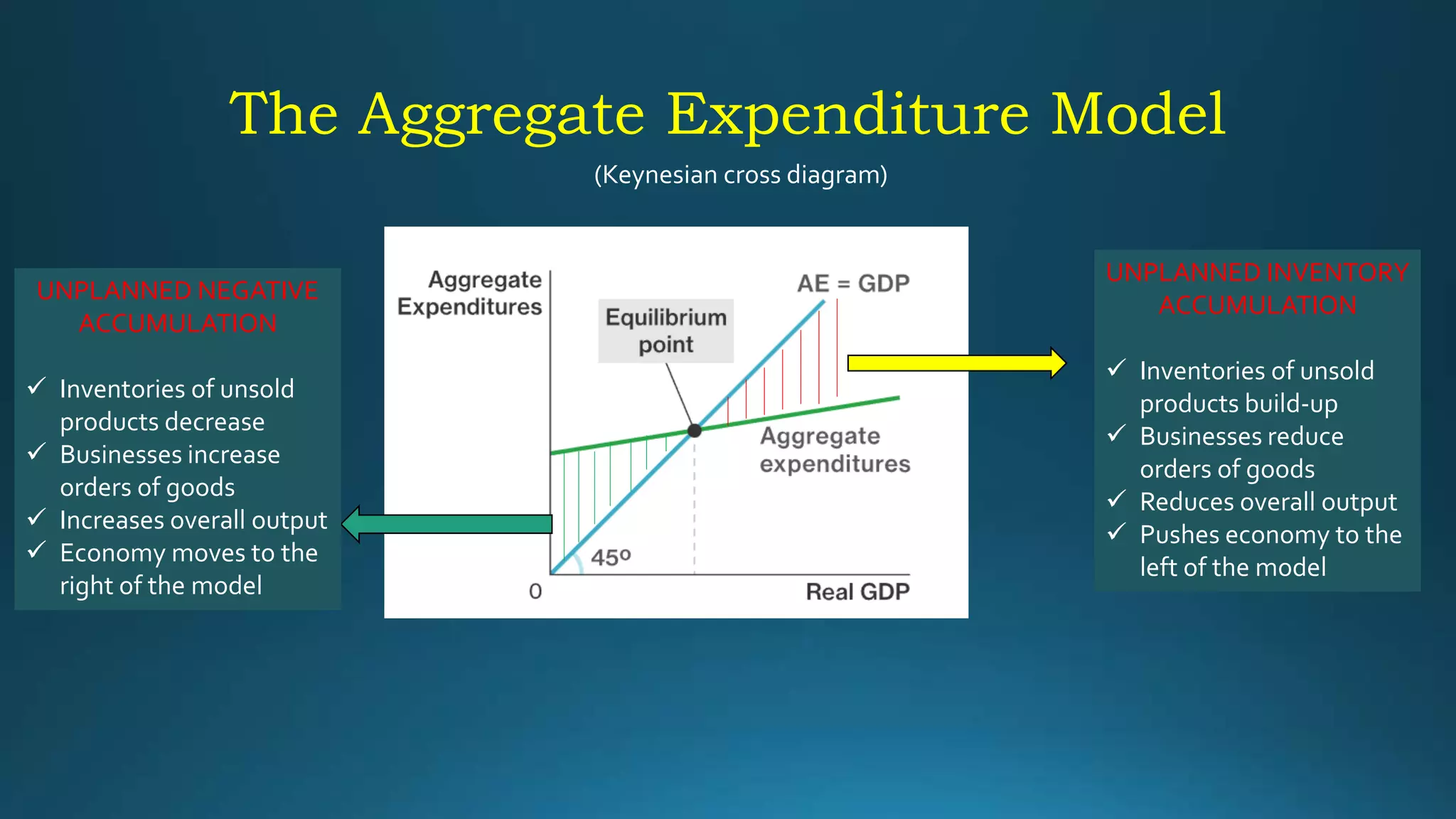
1. The document discusses consumption theory and how consumption relates to income through consumption functions. It defines consumption and savings functions and explains how to calculate them based on different income levels. 2. The aggregate expenditure model is introduced as a way to relate total spending in the economy to gross domestic product. The model shows equilibrium being reached at the point where total expenditures equal GDP, which can be seen via a Keynesian cross diagram. 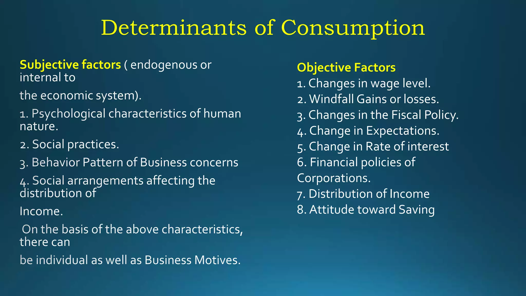3. Determinants of consumption and the calculation of equilibrium output are outlined. Equilibrium output is found using the consumption function equation and setting consumption equal to income to find the level where total expenditures and income are equal

1. CONSUMPTION FUNCTION,
AGGREGATE EXPENDITURE,
AND EQUILIBRIUM OUTPUT
JOJET B.ANDRINO, LPT, MBA (Occ.)
Instructor
LESSON 5

2. OBJECTIVES
 Define the theory of consumption
 Compute the Consumption function and the savings function
 Describe the determinants of consumption
 Examine the aggregate expenditure model
 Calculate Equilibrium Output

3. The Theory of Consumption
Consumption is the act of using resources to satisfy current
needs and wants
Consumption theories began with John Maynard Keynes in 1936
and were developed by economists such as Friedman, Dusenbery,
and Modigliani. The relationship between consumption and
income was a crucial concept in macroeconomic analysis for a
long time.
The consumption function shows how changes in income affect
consumption, with higher income leading to higher consumption,
and vice versa.

4. Keynes’s Psychological Law of
Consumption
Three related Propositions
1.When Income increases, consumption
expenditure also
increases but by a smaller amount.Thus, it
increases less than
proportionately.
2.The increased income will be divided in
some proportion
between consumption expenditure and saving.
3. Increased income always leads to increased
consumption and saving.

5. The Consumption Function

6. Income (y) Consumption (c)
0 20
60 70
120 120
180 170
240 220
300 270
C = a + by
C= 20 + 0.8333 (0)
C= 20 + 0
C = 20
C = a + by
C= 20 + 0.8333 (60)
C= 20 + 49.99
C= 69.99 or 70
C= a + by
C= 20 + 0.8333 (120)
C= 20 + 99.99
C= 119.99 or 120
C = a + by
C= 20 + 0.8333 (180)
C= 20 + 149.99
C = 169.99 or 170
C = a + by
C= 20 + 0.8333 (240)
C= 20 + 199.99
C= 219.99 or 220
C= a + by
C= 20 + 0.8333 (300)
C= 20 + 249.99
C= 269.99 or 270

7. Marginal Propensities to Consume (MPC)
It is defined as the ratio of change in consumption to the
change in income.
MPC is assumed to be positive and less than unity which
means that consumption is an increasing function of income
and it increases by less than the increase of income.
SCHEDULE OF INCOME AND CONSUMPTION

8. Savings Function
The savings function refers to the
standard equation of savings which
defines the relationship between
savings and income where savings
value can be derived at each level with
the use of income value.
S = y – c
Where:
y = Income/Disposable Income
c = consumption
Income (y) Consumption (c) Savings (s)
0 20 (20)
60 70 (10)
120 120 0
180 170 10
240 220 20
300 270 30
SCHEDULE OF INCOME, CONSUMPTION AND
SAVINGS

9. Marginal Propensities to Save
Income (y) Consumption (c) Savings (s)
0 20 (20)
60 70 (10)
120 120 0
180 170 10
240 220 20
300 270 30
SCHEDULE OF INCOME, CONSUMPTION AND
SAVINGS
MPC + MPS
0.8333 + 0.1667 = 1

10. Determinants of Consumption
Subjective factors Objective Factors
1. Changes in wage level.
2.Windfall Gains or losses.
3. Changes in the Fiscal Policy.
4. Change in Expectations.
5. Change in Rate of interest
6. Financial policies of
Corporations.
7. Distribution of Income
8. Attitude toward Saving

11. The Aggregate Expenditure Model
The aggregate expenditure model
relates the components of spending
(consumption, investment,
government purchases, and net
exports) to the level of economic
activity. In the short run, taking the
price level as fixed, the level of
spending predicted by the
aggregate expenditure model
determines the level of economic
activity in an economy.
Figure 16.11
We illustrate this in Figure 16.11 "Planned
Spending in the Aggregate Expenditure
Model" where we suppose for simplicity
that there is a linear relationship between
spending and GDP.

12. The Aggregate Expenditure Model
The aggregate expenditure model is a visual representation of the
relationship between aggregate expenditures and the real gross domestic
product (real GDP), which is the total output of the economy adjusted for
inflation. This relationship is generally shown by a simple graph, where
aggregate expenditures is represented on the vertical axis and real GDP is
represented on the horizontal axis. This graph is also known as a Keynesian
cross diagram. On this graph, there are two observed components. One is
the aggregate expenditure function, which shows how aggregate
expenditures increase as real GDP increases. The aggregate expenditure
function component looks like a line on the graph with a positive slope. The
second component to the aggregate expenditure model is a 45-degree line
that shows where aggregate expenditures (AE) equals real GDP. Graphically
speaking, the coordinates to this line start at the origin (aggregate
expenditures and real GDP both equal zero), and extend outward with a
constant slope of 1 (this way, the coordinates on the line are always equal
each other). The intersection of these two components, the aggregate
expenditure function and the 45-degree line, is the equilibrium point or
equilibrium GDP. The intersection of these two lines must be the equilibrium
because the point of intersection is the definition of GDP (the value, or total
expenditure, of all final goods and services produced within a country's
borders in a given year).This equilibriumGDP is where AE = GDP
The Keynesian cross diagram shows that
aggregate demand increases as output,
measured as real GDP, increases.This
demonstrates the principle of effective
demand.The equilibrium is the point
where aggregate expenditures equal real
GDP, which is shown when the aggregate
expenditures line crosses the 45-degree
line.

13. The Aggregate Expenditure Model
UNPLANNED INVENTORY
ACCUMULATION
 Inventories of unsold
products build-up
 Businesses reduce
orders of goods
 Reduces overall output
 Pushes economy to the
left of the model
UNPLANNED NEGATIVE
ACCUMULATION
 Inventories of unsold
products decrease
 Businesses increase
orders of goods
 Increases overall output
 Economy moves to the
right of the model
(Keynesian cross diagram)

14. Determination of Equilibrium Output
C = a + by (consumption function equation)
Let C =Y
Therefore, the new formula would be:
Y = a + by (use this formula in determining
Equilibrium Point/Output or Break-even Point
Y = a + by
Y = 20 + 0.8333y
Y – 0.8333y = 20 (Transposed)
0.1667 y = 20
0.1667
Y = 20_
0.1667
Y = 199.98 or 120

15. 1 whole yellow paper
Income (y) Consumption (c) Savings (s)
0 50
200
400
600
800
1000
SCHEDULE OF INCOME, CONSUMPTION AND
SAVINGS
1. Compute the consumption (25
points) and savings (12 points)
2. Find the MPS (5 points)
3. Find the Equilibrium Point (10
points)
Plus 3 points
TOTAL Points = 55/55
Note:
• show your solutions
• Use two (2) decimal point
• MPC = 85.5 %