Introduction to FEM
FiniteElement Analysis (ENGR 455)
Dr. Andreas Schiffer
Assistant Professor, Mechanical Engineering
Tel: +971‐(0)2‐4018204
andreas.schiffer@kustar.ac.ae
2.
2
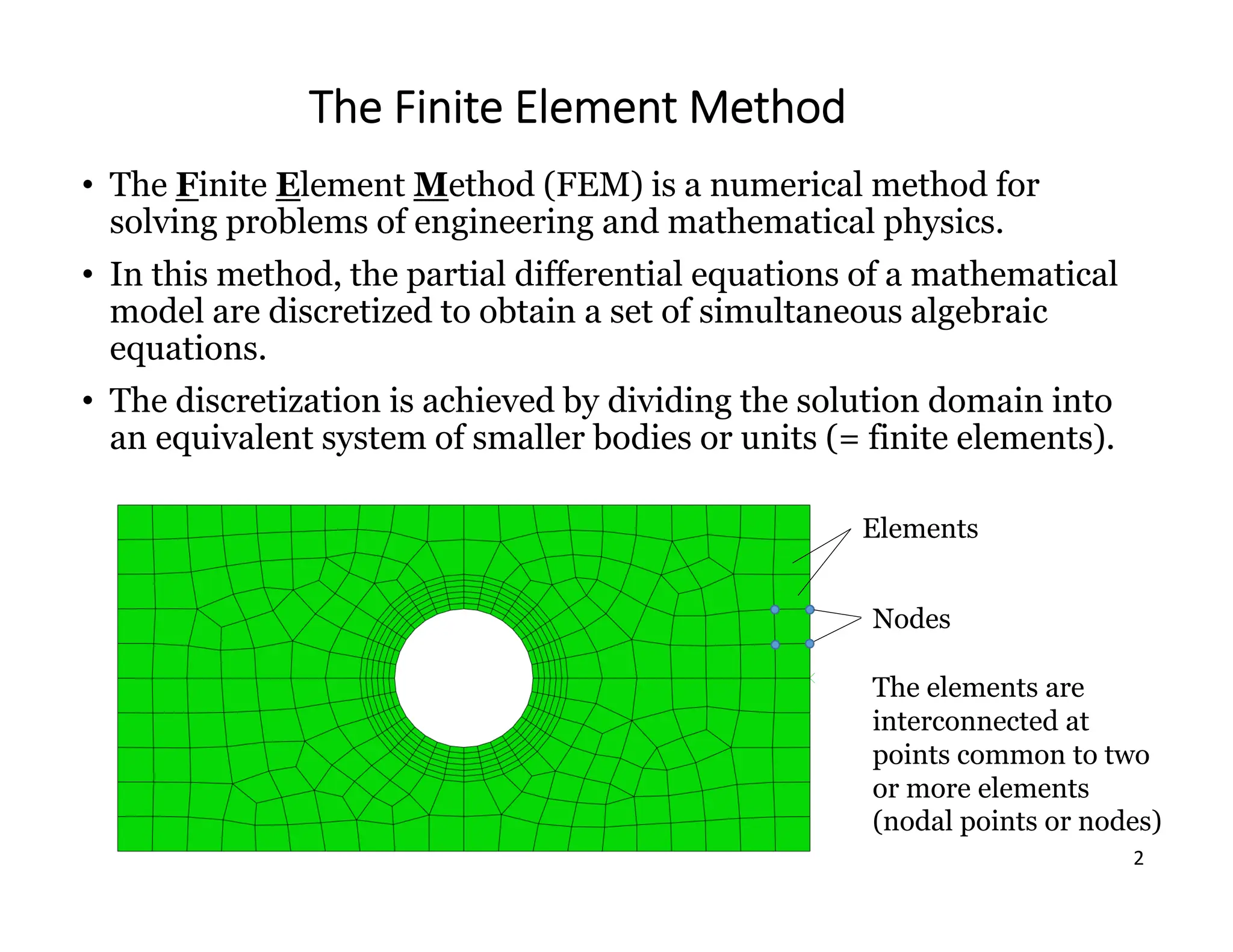
The Finite ElementMethod
• The Finite Element Method (FEM) is a numerical method for
solving problems of engineering and mathematical physics.
• In this method, the partial differential equations of a mathematical
model are discretized to obtain a set of simultaneous algebraic
equations.
• The discretization is achieved by dividing the solution domain into
an equivalent system of smaller bodies or units (= finite elements).
Elements
Nodes
The elements are
interconnected at
points common to two
or more elements
(nodal points or nodes)
3.
3
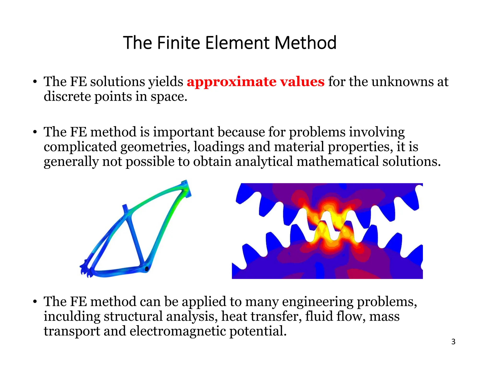
The Finite ElementMethod
• The FE solutions yields approximate values for the unknowns at
discrete points in space.
• The FE method is important because for problems involving
complicated geometries, loadings and material properties, it is
generally not possible to obtain analytical mathematical solutions.
• The FE method can be applied to many engineering problems,
inculding structural analysis, heat transfer, fluid flow, mass
transport and electromagnetic potential.
4.
4
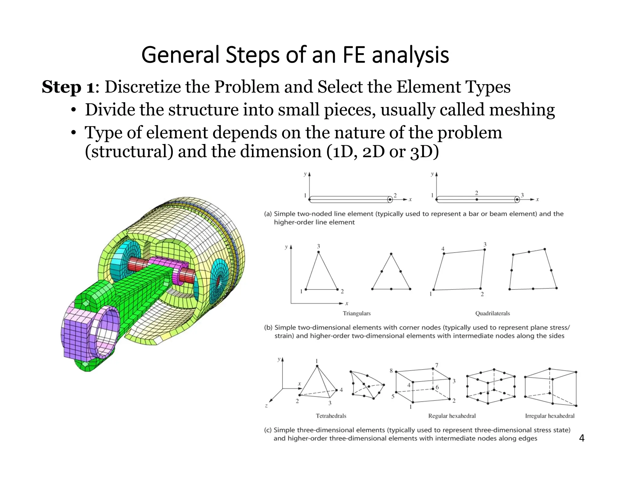
General Steps ofan FE analysis
Step 1: Discretize the Problem and Select the Element Types
• Divide the structure into small pieces, usually called meshing
• Type of element depends on the nature of the problem
(structural) and the dimension (1D, 2D or 3D)
5.
5
General Steps ofan FE analysis
Step 2: Select a Displacement Function
• Choosing a displacement function within each element
connecting the nodes.
• Linear, quadratic and cubic polynomials are most common.
Step 3: Define the Stress-Strain Relationships
• Describe the constitutive law relating stresses to strains in each
element
• The simplest constitutive relation is Hooke’s law,
σx = E εx (in 1D).
Step 4: Derive the Element Stiffness Matrix and Equations
• Write the system of equations describing the structural behavior
of an element.
• Relating nodal forces to nodal displacements of the element
through an element stiffness matrix:
f k d
6.
6
General Steps ofan FE analysis
Step 5: Assemble the Global System Equation
• All individual elements are assembled using the method of
superposition (or direct stiffness method) to produce the global or
total system of equations of the problem.
Here, {F} is the vector of global nodal forces, [K] is the structure
global or total stiffness matrix, {d} is now the vector of known and
unknown structure nodal degrees of freedom (displacements).
• It can be shown that at this stage, the global stiffness matrix [K] is
a singular square matrix because its determinant is equal to zero.
• To remove this singularity, we must invoke certain boundary
conditions (or constraints or supports) so that the structure
remains in place instead of moving as a rigid body.
• Step 6: Apply Boundary Conditions and Loading
• Prescribe forces and displacements at nodes.
F K d
F K d
7.
7
General Steps ofan FE analysis
• Step 7: Solve for the Unknown Degrees of Freedom
• Involves finding the inverse of the global stiffness matrix [K]-1 .
• Then the structure’s unknown nodal degrees of freedom {d} can
be calculated via
• Step 8: Solve for the Element Strains and Stresses
• Strains can be directly expressed in terms of the displacements
determined in Step 7.
• Stresses are obtained from the strain solutions through the
constitutive law (e.g. Hooke’s law).
• Step 9: Interpret the Results (Post-processing)
Determination of locations in the structure where large deformations
and large stresses occur is generally important in making design
decisions.
1. Pre-processing (Step 1-6)
2. Solution (Step 7-8)
3. Post-processing (Step 9)
1
d K F
There are 3 categories of
steps in an FE analysis:
F K d
8.
8
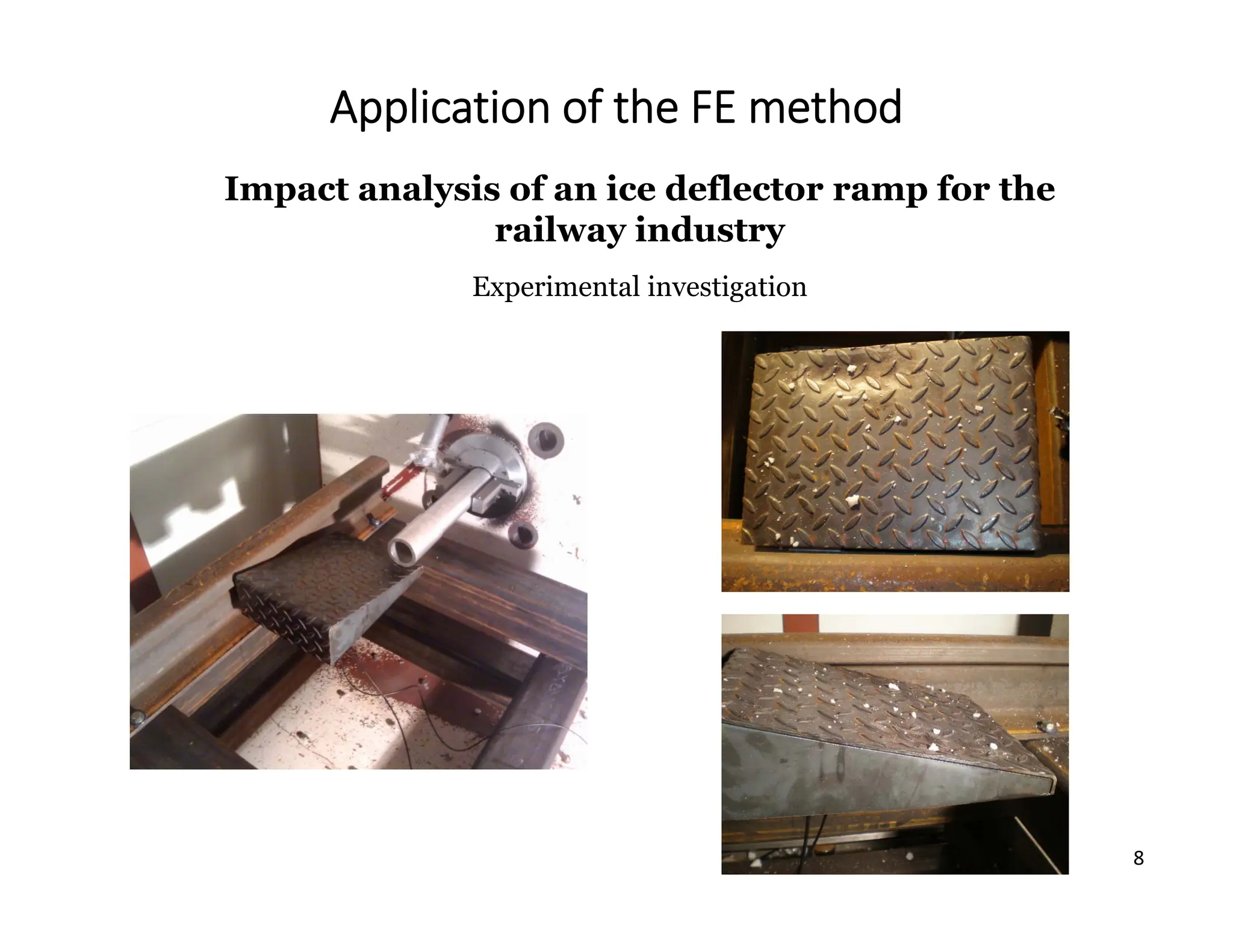
Application of theFE method
Impact analysis of an ice deflector ramp for the
railway industry
Experimental investigation
9.
9
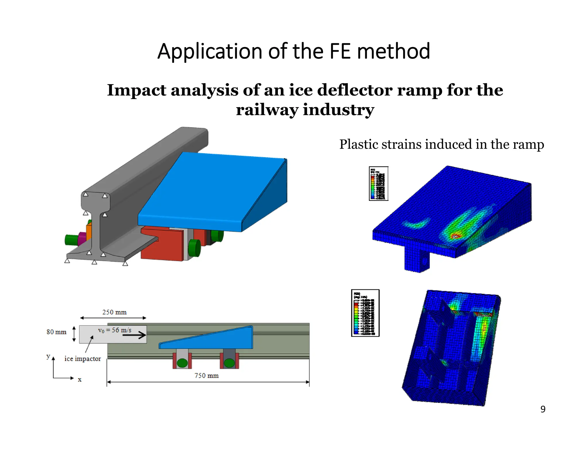
Application of theFE method
Impact analysis of an ice deflector ramp for the
railway industry
Plastic strains induced in the ramp
10.
10
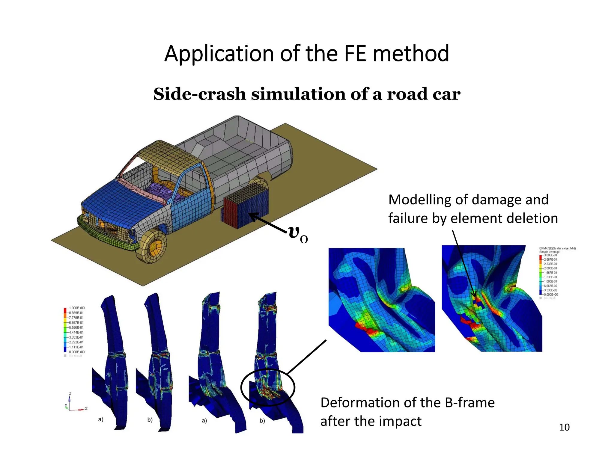
Application of theFE method
Side-crash simulation of a road car
v0
Deformation of the B‐frame
after the impact
Modelling of damage and
failure by element deletion
11.
11
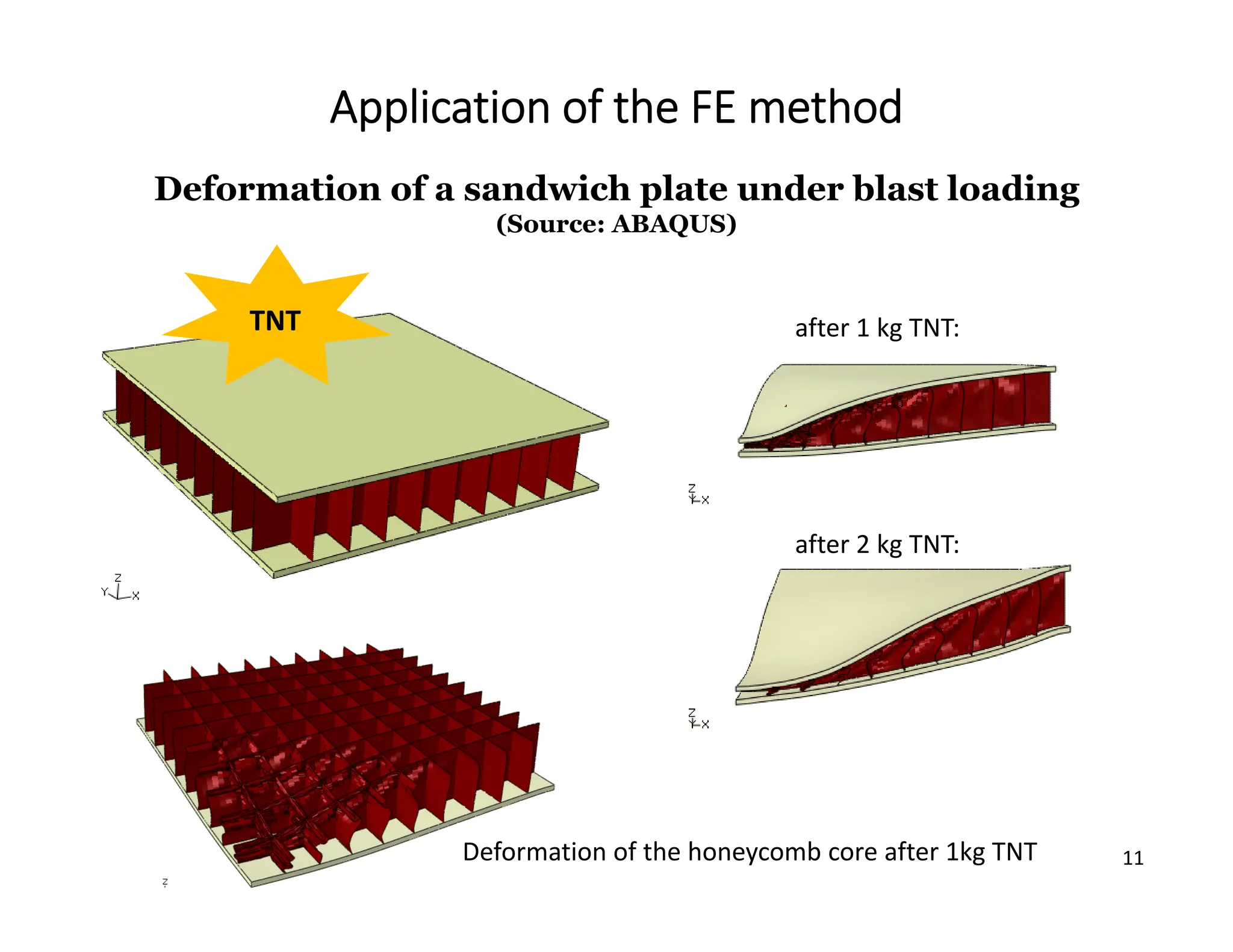
Application of theFE method
Deformation of a sandwich plate under blast loading
(Source: ABAQUS)
TNT after 1 kg TNT:
after 2 kg TNT:
Deformation of the honeycomb core after 1kg TNT
12.
12
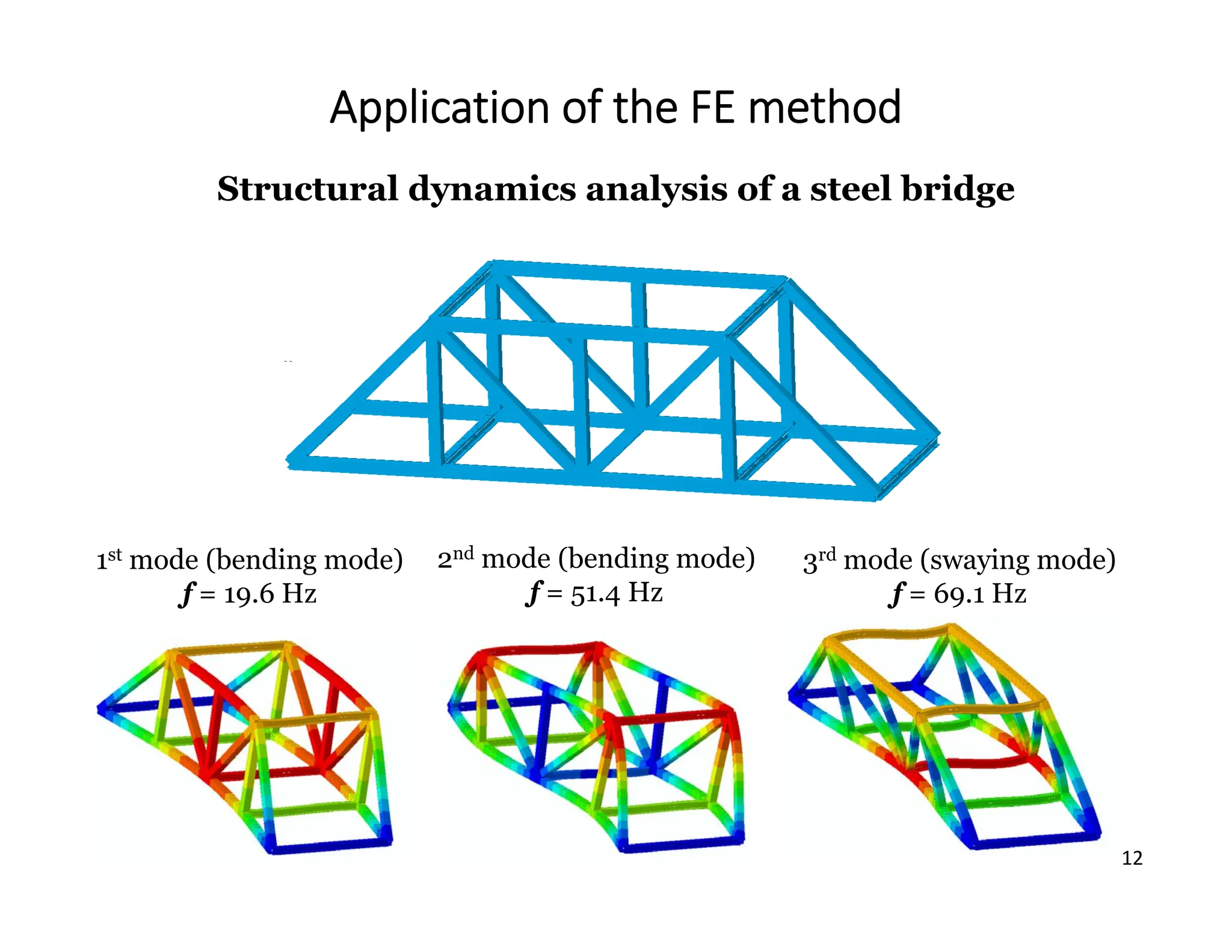
Application of theFE method
Structural dynamics analysis of a steel bridge
1st mode (bending mode)
f = 19.6 Hz
2nd mode (bending mode)
f = 51.4 Hz
3rd mode (swaying mode)
f = 69.1 Hz
13.
13
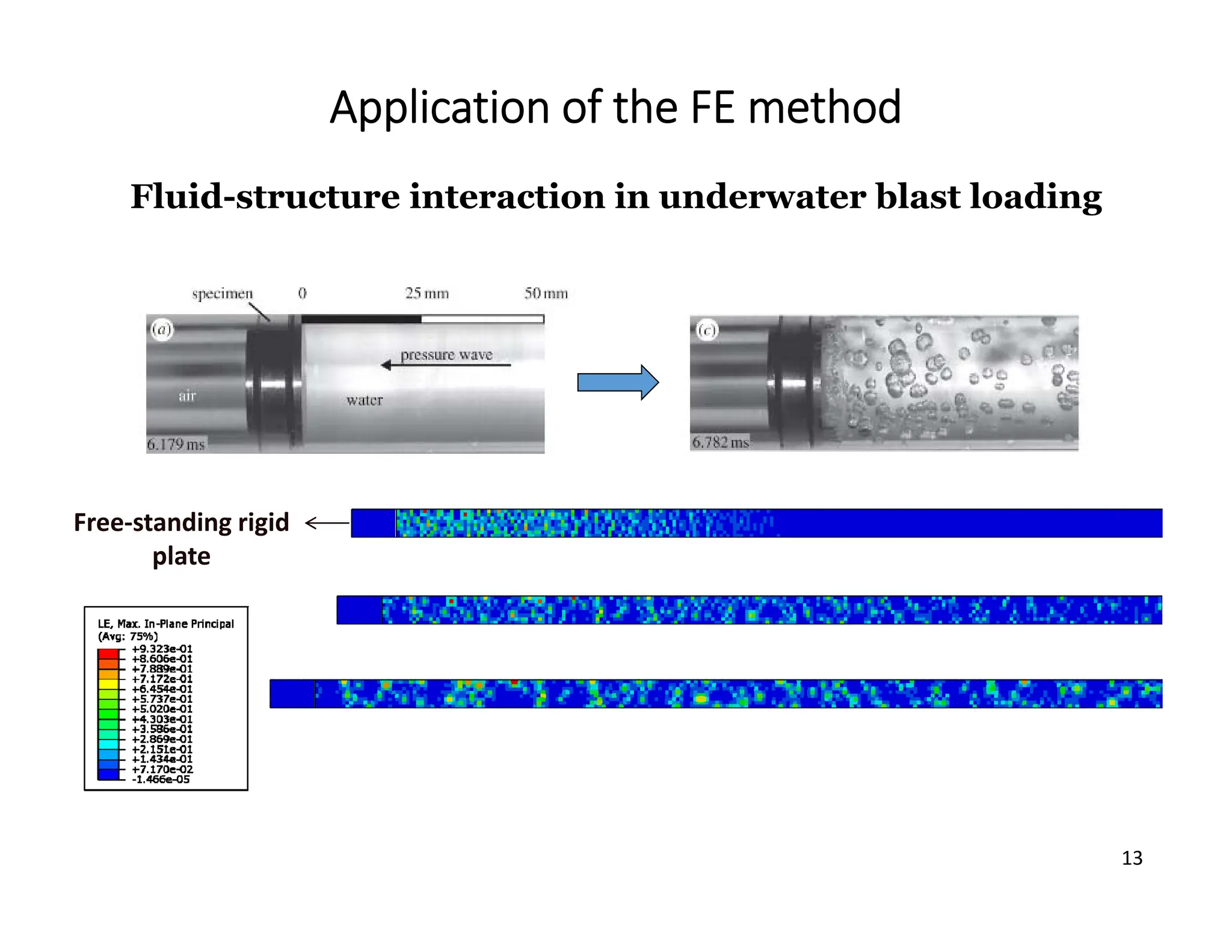
Application of theFE method
Fluid-structure interaction in underwater blast loading
Free‐standing rigid
plate
14.
14
Application of theFE method
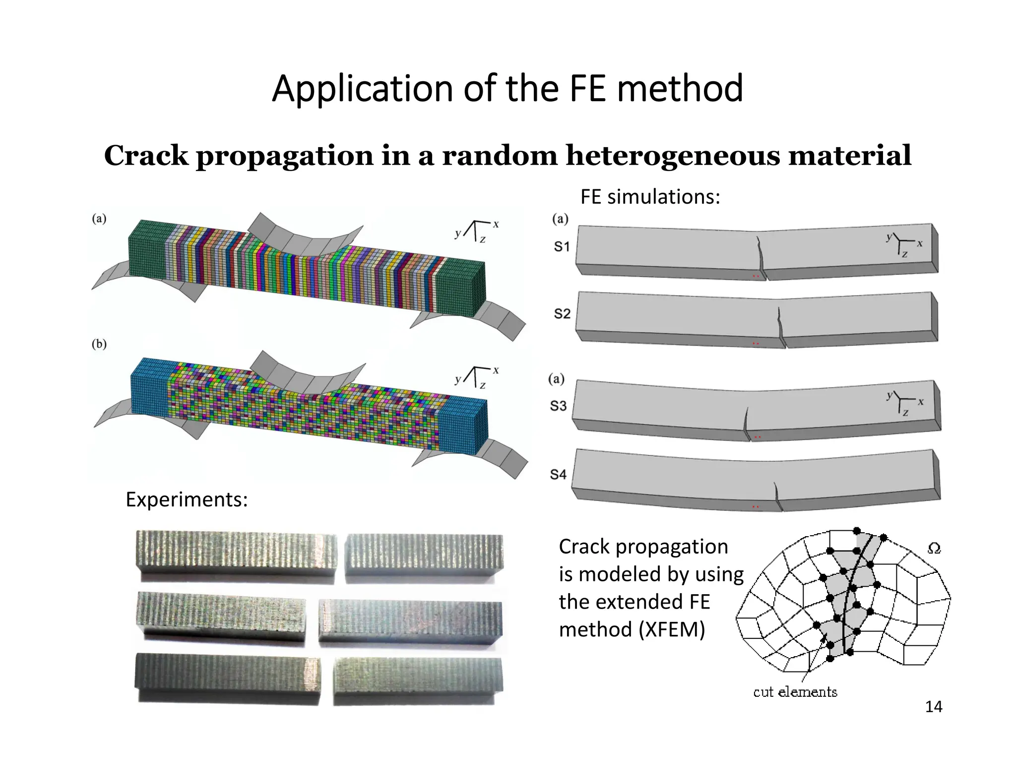
Crack propagation in a random heterogeneous material
Crack propagation
is modeled by using
the extended FE
method (XFEM)
Experiments:
FE simulations:

![6
General Steps of an FE analysis
Step 5: Assemble the Global System Equation
• All individual elements are assembled using the method of
superposition (or direct stiffness method) to produce the global or
total system of equations of the problem.
Here, {F} is the vector of global nodal forces, [K] is the structure
global or total stiffness matrix, {d} is now the vector of known and
unknown structure nodal degrees of freedom (displacements).
• It can be shown that at this stage, the global stiffness matrix [K] is
a singular square matrix because its determinant is equal to zero.
• To remove this singularity, we must invoke certain boundary
conditions (or constraints or supports) so that the structure
remains in place instead of moving as a rigid body.
• Step 6: Apply Boundary Conditions and Loading
• Prescribe forces and displacements at nodes.
F K d
F K d
](https://image.slidesharecdn.com/282165203-module-1-introduction-to-fem-250809232933-1709c3e2/75/282165203-Module-1-Introduction-to-FEM-pdf-6-2048.jpg)
![7
General Steps of an FE analysis
• Step 7: Solve for the Unknown Degrees of Freedom
• Involves finding the inverse of the global stiffness matrix [K]-1 .
• Then the structure’s unknown nodal degrees of freedom {d} can
be calculated via
• Step 8: Solve for the Element Strains and Stresses
• Strains can be directly expressed in terms of the displacements
determined in Step 7.
• Stresses are obtained from the strain solutions through the
constitutive law (e.g. Hooke’s law).
• Step 9: Interpret the Results (Post-processing)
Determination of locations in the structure where large deformations
and large stresses occur is generally important in making design
decisions.
1. Pre-processing (Step 1-6)
2. Solution (Step 7-8)
3. Post-processing (Step 9)
1
d K F
There are 3 categories of
steps in an FE analysis:
F K d
](https://image.slidesharecdn.com/282165203-module-1-introduction-to-fem-250809232933-1709c3e2/75/282165203-Module-1-Introduction-to-FEM-pdf-7-2048.jpg)