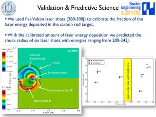
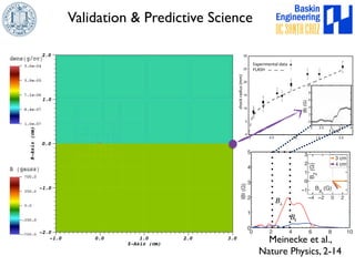
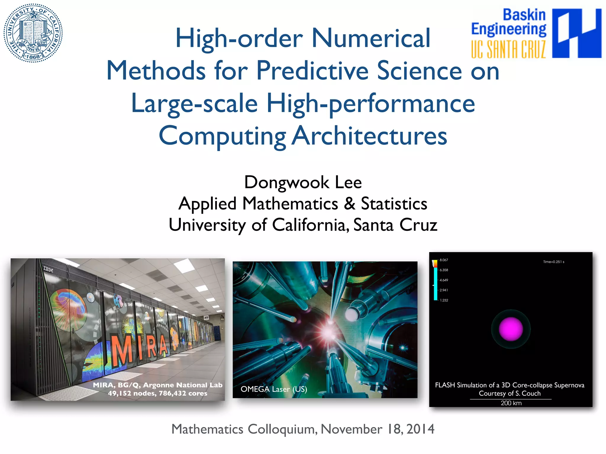
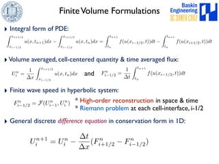
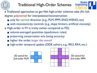
This document discusses high-order numerical methods for predictive science on large-scale high-performance computing architectures. It covers three main topics: 1) High performance computing and how modern architectures have increasing numbers of cores but declining memory per core, requiring a shift in numerical algorithms. 2) Ideas on high-order numerical methods that are more accurate using less grid points and higher-order approximations. 3) The importance of validating and verifying simulations against theoretical solutions and experiments for predictive science.

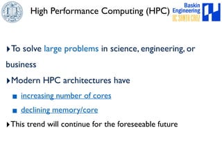
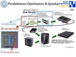
![1. Mathematical Models
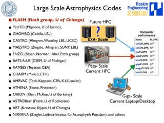
Hydrodynamics (gas dynamics)
@⇢
@t
+ r · (⇢v) = 0 mass eqn
@⇢v
@t
+ r · (⇢vv) + rP = ⇢g momentum eqn
@⇢E
@t
+ r · [(⇢E + P)v] = ⇢v · g total energy eqn
P = (! 1)⇢✏
E = ✏ +
1
2|v|2
@⇢✏
@t
+ r · [(⇢✏ + P)v] − v · rP = 0
Equation of State](https://image.slidesharecdn.com/dongwookleemathucsc-141119143521-conversion-gate01/85/Mathematics-Colloquium-UCSC-19-320.jpg)
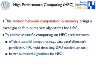
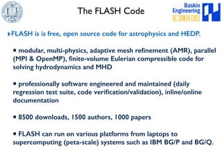
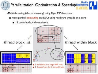
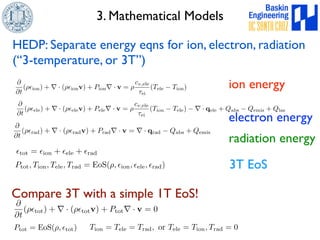
![2. Mathematical Models
Magnetohydrodynamics (MHD)
@⇢
@t
+ r · (⇢v) = 0 mass eqn
@⇢v
@t
+ r · (⇢vv − BB) + rP⇤ = ⇢g + r · ⌧ momentum eqn
@⇢E
@t
+ r · [v(⇢E + P⇤) − B(v · B)] = ⇢g · v + r · (v · ⌧ + $rT) + r · (B ⇥ (⌘r⇥B))
total energy eqn
@B
@t
+ r · (vB − Bv) = −r ⇥ (⌘r⇥B) induction eqn
P⇤ = p +
B2
2
E =
v2
2
+ ✏ +
B2
2⇢
Equation of State
⌧ = μ[(rv) + (rv)T −
2
3
solenodidal constraint
(r · v)I]
viscosityr · B = 0](https://image.slidesharecdn.com/dongwookleemathucsc-141119143521-conversion-gate01/85/Mathematics-Colloquium-UCSC-20-320.jpg)
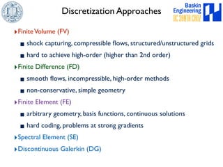
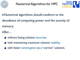
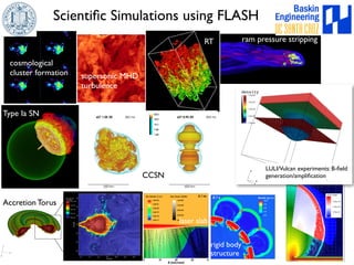
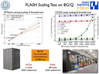
![Unsplit FV Formulation
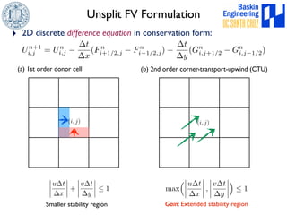
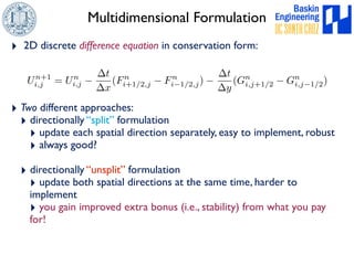
‣ 2D discrete difference equation in conservation form:
Un+1
i,j = Un
i,j
ut
x
[Un
i,j Un
i1,j ]
vt
y
[Un
i,j1] Un+1
i,j Un
i,j = Un
i,j
ut
x
[Un
i,j Un
i1,j ]
vt
y
[Un
i,j Un
i,j1]
+
t2
2
n u
x
⇥ v
y
(Un
i,j Un
i,j1)
v
y
(Un
i1,j Un
i1,j1)
⇤
+
v
y
⇥ v
y
(Un
i,j Un
i1,j)
v
y
(Un
i,j1 Un
i1,j1)
⇤o
Extra cost for corner coupling!
(a) 1st order donor cell
(i, j)
Un+1
i,j = Un
i,j
t
x
(Fn
i+1/2,j Fn
i1/2,j)
t
y
(Gn
i,j+1/2 Gn
i,j1/2)
(b) 2nd order corner-transport-upwind (CTU)
(i, j)](https://image.slidesharecdn.com/dongwookleemathucsc-141119143521-conversion-gate01/85/Mathematics-Colloquium-UCSC-40-320.jpg)