ekonometrika

1. Center for Teaching, Research & Learning
Social Science Research Lab
American University, Washington, D.C.
http://www.american.edu/provost/ctrl/
202-885-3862
Stata & Time series
Stata is a general-purpose statistical software package. Stata's full range of capabilities include: data
management, statistical analysis, graphics, simulations, and custom programming.
Course Objective
This course is designed to give a basic understanding of some of the features available in Stata
when working with time series analysis. Time series data represents a pool of variables observed
and recorded over time. For this tutorial we are going to use the “Time series.dta” data set
containing the following variables: date, unemployment, consumer price index (CPI), interest
rate, and GDP growth. “Time series.dta” contains observations for each quarter from 1960 to
2005.
Learning Outcomes
1. Opening the data set and data description
2. Declaring the data to be Time Series
3. Useful time series command
4. Autocorrelation and cross-correlation analysis
5. Unit Root test
1. Opening the data set and data description
We recommend that you create a log file before you start working in Stata, this way you will
have all your computations on a file to review afterwards.
To do this, go to: File > Log > Begin. This file will record all the input that you type, as well as all
the output produced by STATA. Alternatively, you can type (in the command window):
log using "C:UsersCTRLDesktopTSlog.log"

2. Opening the data file. For this tutorial, we will use Time series.dta, which can be downloaded
from:
http://www.american.edu/provost/ctrl/trainingguides.cfm.
In Stata 11 and earlier versions, before you open the dataset, you may need to set the memory
size. (In this instance, this isn’t necessary, as the example dataset is relatively small and does not
require a lot of memory.) To tell STATA how much memory to set aside for data, type:
set mem 100m
(This command is not needed in Stata 12)
Once you have downloaded and unzipped the dataset, you can access by going to: File > Open.
Alternatively, you can type:
use "C:UsersCTRLDesktopTime series.dta", clear
where the clear option has been appended. This clears Stata’s memory, allowing you to open a
new dataset.
In order to get a sense of what the data file contains we can use a couple of commands:
summerize and describe, both stata commands provide useful information about our data set
and variables.
Summarize calculates and displays a variety of univariate summary statistics. If no variable list is
specified, summary statistics are calculated for all the variables in the dataset.
Describe produces a summary of the dataset in memory or of the data stored in a Stata-format
dataset.
Example using “Time series.dta”
summarize
datevar 181 90 52.39434 0 180
gdp 181 2.031231 2.001162 -1.703726 9.718504
interest 181 6.167403 3.3706 .98 19.1
cpi 181 95.91184 54.13317 29.39667 192.1667
unemp 181 5.914917 1.453928 3.4 10.66667
Variable Obs Mean Std. Dev. Min Max

3. describe
2. Declaring the data to be Time Series
Using the time variable “datevar”, we are able to declare the data as times series in order to use
the time series operators.
Using the tsset command
tsset declares the data in memory to be a time series. tssetting the data is what makes Stata's
time-series operators such as L. and F. (lag and lead) work. Also, before using the other time -
series commands, you must tsset the data first. If you save the data after tsset, Stata will
remember that data as being time series and you will not have to tsset again.
Example using “Time series.dta”
tsset datevar
Note: dataset has changed since last saved
Sorted by: datevar
datevar float %tq Date variable
gdp float %9.0g GDP annual growth
interest float %9.0g Federal Funds Interest Rate
cpi float %9.0g Consumer Price Index
unemp float %9.0g Unemployment Rate
variable name type format label variable label
storage display value
size: 3,620
vars: 5 12 Oct 2011 10:00
obs: 181
Contains data from C:UsersCTRLDesktopTime series.dta
delta: 1 quarter
time variable: datevar, 1960q1 to 2005q1

4. 3. Useful Time Series commands
In this section, we introduce a few basic but very helpful commands.
tin (times in, from time A to time B) option:
list datevar unemp if tin(2000q1,2000q4)
twithin (times within time A and time B, excluding the two time points) option:
list datevar unemp if twithin(2001q1,2001q3)
164. 2000q4 3.9
163. 2000q3 4
162. 2000q2 3.933333
161. 2000q1 4.033333
datevar unemp
166. 2001q2 4.4
datevar unemp

5. Generating values bases on past observations using the lag operator and forward-looking values
using the lead operator:
generate unempL1=L1.unemp
generate unempL2=L2.unemp
list datevar unemp unempL1 unempL2 in 1/5
generate unempF1=F1.unemp
generate unempF2=F2.unemp
list datevar unemp unempF1 unempF2 in 1/5
5. 1961q1 6.8 6.266667 5.533333
4. 1960q4 6.266667 5.533333 5.233333
3. 1960q3 5.533333 5.233333 5.133333
2. 1960q2 5.233333 5.133333 .
1. 1960q1 5.133333 . .
datevar unemp unempL1 unempL2
5. 1961q1 6.8 7 6.766667
4. 1960q4 6.266667 6.8 7
3. 1960q3 5.533333 6.266667 6.8
2. 1960q2 5.233333 5.533333 6.266667
1. 1960q1 5.133333 5.233333 5.533333
datevar unemp unempF1 unempF2

6. To generate the difference between current and previous values, use the D operator. The
transformations are as follows: D1 = Yt – Yt-1 and D2 = (Yt–Yt-1) – (Yt-1–Yt-2).
generate unempD1=D1.unemp
generate unempD2=D2.unemp
list datevar unemp unempD1 unempD2 in 1/5
4. Autocorrelation and cross-correlation analysis
In this section, we show you how to explore autocorrelation and cross-correlation.
Autocorrelation represent the correlation between a variable and its previous values; use the ac
and pac commands. To explore the relationship between two time series, use the command
xcorr, making sure that you always list the independent variable first and the dependent
variable second.
ac produces a correlogram (a graph of autocorrelations) with pointwise confidence intervals
that is based on Bartlett's formula for MA(q) processes.
pac produces a partial correlogram (a graph of partial autocorrelations) with confidence
intervals calculated using a standard error of 1/sqrt(n). The residual variances for each lag may
optionally be included on the graph.
xcorr plots the sample cross-correlation function.
5. 1961q1 6.8 .5333333 -.2000003
4. 1960q4 6.266667 .7333336 .4333334
3. 1960q3 5.533333 .3000002 .2000003
2. 1960q2 5.233333 .0999999 .
1. 1960q1 5.133333 . .
datevar unemp unempD1 unempD2

7. Example using “Time series.dta”
ac unemp, lags(10)
In this case, the autocorrelation graph indicates that unemployment is correlated with up to
eight previous quarters.
-0.50
0.000.501.00
0 2 4 6 8 10
Lag
Bartlett's formula for MA(q) 95% confidence bands

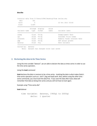
8. pac unemp, lags(10)
xcorr gdp unemp
-1.00-0.50
0.000.501.00
0 2 4 6 8 10
Lag
95% Confidence bands [se = 1/sqrt(n)]
-1.00-0.500.000.501.00
-1.00-0.50
0.000.501.00
-20 -10 0 10 20
Lag
Cross-correlogram

9. The graph above indicates that GDP has a negative correlation with unemployment (six to nine
months).
5. Unit Root test
In this section, we demonstrate how to evaluate if the series has a unit root.
When working with times series data sets it is important to look for unit root. If unit root is
found in a series this means that more than one trend is present in the series.
Let’s look at unemployment across time and test for unit root.
line unemp datevar
468
1012
UnemploymentRate
1960q1 1965q1 1970q1 1975q1 1980q1 1985q1 1990q1 1995q1 2000q1 2005q1
Date variable

10. In order to assess for Unit Root we can use the Dickey-Fuller test to examine for stochastic
trends, using the following command:
dfuller unemp, lag(5)
In this case the null hypothesis is that unemployment has a unit root. The Z-score yielded by the
test shows that unemployment has a unit root, because it falls within the acceptance interval
(i.e. |-2.597| < |-3.481|).
When testing for unit root on the first difference of unemployment, we will find out that it does
not have unit root:
dfuller unempD1, lag(5)
In this case The Z-score does not fall within the acceptance interval (i.e. |-5.303| > |-3.481|)
therefore we can discard a unit root.
MacKinnon approximate p-value for Z(t) = 0.1201
Z(t) -2.481 -3.485 -2.885 -2.575
Statistic Value Value Value
Test 1% Critical 5% Critical 10% Critical
Interpolated Dickey-Fuller
Augmented Dickey-Fuller test for unit root Number of obs = 175
MacKinnon approximate p-value for Z(t) = 0.0001
Z(t) -4.593 -3.485 -2.885 -2.575
Statistic Value Value Value
Test 1% Critical 5% Critical 10% Critical
Interpolated Dickey-Fuller
Augmented Dickey-Fuller test for unit root Number of obs = 174