1. The International Journal Of Engineering And Science (IJES)
||Volume||2 ||Issue|| 5 ||Pages|| 46-56||2013||
ISSN(e): 2319 – 1813 ISSN(p): 2319 – 1805
www.theijes.com The IJES Page 46
A New Jpeg Image Scaling Algorithm Based on the Area Pixel
Model
1,
Sourabh Jain MTech , 2,
Prof D. Suresh
1,
Sem, Set, Jain University
Under The Guidance Of
2
,Dept Of Ece ,Set ,Jain University
--------------------------------------------------ABSTRACT--------------------------------------------------------
Image scaling is a very important technique and has been widely used in many image processing applications.
In this paper, we present an edge-oriented area-pixel scaling processor. To achieve the goal of low cost, the
area-pixel scaling technique is implemented with a low-complexity VLSI architecture in our design. A simple
edge catching technique is adopted to preserve the image edge features effectively so as to achieve better image
quality. Compared with the previous low-complexity techniques, our method performs better in terms of both
quantitative evaluation and visual quality. The seven-stage VLSI architecture of our image scaling processor
contains 10.4-K gate counts and yield a processing rate of about 200 MHz by using TSMC 0.18- m technology.
--------------------------------------------------------------------------------------------------------------------------------------
Date of Submission: 01,May ,2013 Date of Publication: 5.June,2013
--------------------------------------------------------------------------------------------------------------------------------------
I. INTRODUCTION
IMAGE scaling is widely used in many fields ranging from consumer electronics to medical imaging.
It is indispensable when the resolution of an image generated by a source device is different from the screen
resolution of a target display. For example, we have to enlarge images to fit HDTV or to scale them down to fit
the mini-size portable LCD panel. The most simple and widely used scaling methods are the nearest neighbour
and bilinear techniques. In recent years, many efficient scaling methods have been proposed in the literature .
According to the required computations and memory space, we can divide the existing scaling methods into two
classes: lower complexity and higher complexity scaling techniques. The complexity of the former is very low
and comparable to conventional bilinear method. The latter yields visually pleasing images by utilizing more
advanced scaling methods. In many practical real-time applications, the scaling process is included in end-user
equipment, so a good lower complexity scaling technique, which is simple and suitable for low-cost VLSI
implementation, is needed. In this paper, we consider the lower complexity scaling techniques only.
Kim et al. presented a simple area-pixel scaling method. It uses an area-pixel model instead of the
common point-pixel model and takes a maximum of four pixels of the original image to calculate one pixel of a
scaled image. By using the area coverage of the source pixels from the applied mask in combination with the
difference of luminosity among the source pixels, Andreadis et al. [8] proposed a modified area-pixel scaling
algorithm and its circuit to obtain better edge preservation. Both Bilinear and Bicubic obtain better edge-
preservation but require about two times more of computations than the bilinear method. To achieve the goal of
lower cost, we present an edge-oriented area-pixel scaling processor in this paper. The area-pixel
scaling technique is approximated and implemented with the proper and low-cost VLSI circuit in our
design. The proposed scaling processor can support floating-point magnification factor and preserve the edge
features efficiently by taking into account the local characteristic existed in those available source pixels around
the target pixel. Furthermore, it handles streaming data directly and requires only small amount of memory: one
line buffer rather than a full frame buffer. The experimental results demonstrate that the proposed design
performs better than other lower complexity image scaling methods in terms of both quantitative evaluation and
visual quality.The seven-stage VLSI architecture for the proposed design was implemented and synthesized by
using Verilog HDL and synopsys design compiler, respectively. In our simulation, the circuit can achieve 200
MHz with 10.4-K gate counts by using TSMC 0.18- m technology. Since it can process one pixel per clock
cycle, it is quick enough to process a video resolution
of WQSXGA (3200 2048) at 30 f/s in real time.

2. A New Jpeg Image Scaling Algorithm...
www.theijes.com The IJES Page 47
This paper is organized as follows. In Section II, the area- pixel scaling technique is introduced briefly. Our
method is presented in Section III. Section IV describes the proposed VLSI architecture in detail. Section V
illustrates the simulation results and chip implementation. The conclusion is provided in Section VI.
II. AREA-PIXEL SCALING TECHNIQUE
A. An Overview of Area-Pixel Scaling Technique
Assume that the source image represents the original image to be scaled up/down and target image
represents the scaled image. The area-pixel scaling technique performs scale-up scale-down transformation by
using the area pixel model instead of the common point model. Each pixel is treated as one small rectangle but
not a point; its intensity is evenly distributed in the rectangle area. Fig. 1 shows an example of image scaleup
process of the area-pixel model where a source image of 4×4 pixels is scaled up to the target image of 5×5
pixels. Obviously, the area of a target pixel is less than that of a source pixel. A window is put on the current
target pixel to calculate its estimated luminance value. As shown in Fig. 1(c), the number of source pixels
overlapped by the current target pixel window is one, two, or a maximum of four. Let the luminance values of
four source pixels overlapped by the window of current target pixel at coordinate (k,l)be denoted as FS(m,n),
FS(m+1,n) and FS(m+1,n+1) respectively. The estimated value of current target pixel, denoted FT ((k,l) can be
calculated by weighted averaging the luminance values of four source pixels with area coverage ratio as
FT ((k,l) = 0
1
∑∑[Fs(m+I,n+j)×W(m+I,n+j)]
Fig 1 (a) source image of 4×4 pixels. (b) A target image of 5×5 pixels. (c) Relations of the target pixel and
source pixels
where W(m,n),W(m+1,n),W(m,n+1) and W(m+1,n+1) represent the weight factors of neigh boring source
pixels for the current target pixel at(k,l) . Assume that the regions of four source pixels overlapped by current
target pixel window are denoted as A(m,n) , A(m+1,n) ,A(m,n+1) and A(m+1,n+1) respectively, and the area of
the target pixel window is denoted as Asum . The weight factors of four source pixels can be given as
[W(m,n),W(m+1,n),W(m,n+1) and W(m+1,n+1) ] = [A(m,n)/ Asum,A(m+1,n)/ Asum,A(m,n+1)/ Asum ,
A(m+1,n+1)/ Asum ] (2)
Where Asum = A(m,n)+A(m+1,n)+A(m,n+1) + A(m+1,n+1)
Let the width and height of the overlapped region A(m,n) be denoted as left‟(k,l)and top‟(k,l) , and the width
and height of A(m+1,n+1) be denoted as right‟(k,l) and bottom‟(k,l), respectively, as shown in Fig. 1(c). Then,
the areas of the overlapped region can be calculated
[A(m,n),A(m+1,n),A(m,n+1) , A(m+1,n+1)] = [left‟(k,l)×top‟(k,l) , right‟(k,l)×top‟(k,l),left‟(k,l)×bottom‟(k,l),
right‟(k,l) × bottom‟(k,l)]. (3)
Obviously, many floating-point operations are needed to determine the four parameters left‟(k,l)top‟(k,l) ,
right‟(k,l) and bottom‟(k,l), if the direct area-pixel implementation is adopted.

3. A New Jpeg Image Scaling Algorithm...
www.theijes.com The IJES Page 48
III THE PROPOSED LOW COMPLEXITY ALGORITHM
Observing (1)–(3), we know that the direct implementation of area-pixel scaling requires some
extensive floating-point computations for the current target pixel at (k,l) to determine the four parameters,
left‟(k,l),top‟(k,l) , right‟(k,l) and bottom‟(k,l), . In the proposed processor, we use an approximate technique
suitable for low-cost VLSI implementation to achieve that goal properly. We modify (3) and implement the
calculation of areas of the overlapped regions as
[A‟(m,n),A‟(m+1,n),A‟(m,n+1) , A‟(m+1,n+1)] = [left‟(k,l)×top‟(k,l) ,
right‟(k,l)×top‟(k,l),left‟(k,l)×bottom‟(k,l), right‟(k,l) × bottom‟(k,l)]. (4)
Those left‟(k,l),top‟(k,l) , right‟(k,l) and bottom‟(k,l)are all 6-b integer and given as
[left‟(k,l),top‟(k,l) , right‟(k,l) , bottom‟(k,l)]=Appr [left‟(k,l),top‟(k,l) ,
right‟(k,l), bottom‟(k,l)] (5)
Where Appr represents the approximate operator adopted in our design and will be explained in detail later. To
obtain better visual quality, a simple low-cost edge catching technique is employed to preserve the edge features
effectively by taking into account the local characteristic existed in
those available source pixels around the target pixel. The final areas of the overlapped regions are given as
[A‟‟(m,n),A‟‟(m+1,n),A‟‟(m,n+1) , A‟‟(m+1,n+1)]= ( [A‟(m,n),A‟(m+1,n),A‟(m,n+1) , A‟(m+1,n+1)]
(6)where we adopt a tuning operator to tune the areas of four overlapped regions according to the edge
features obtained by our edge-catching technique. By applying (6) to (1) and (2),
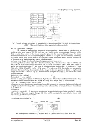
we can determine the estimated luminance value of the current target pixel. Fig. 2 shows the pseudo code of our
scaling method. In the rest of this section, the approximate technique adopted in our design is introduced first.
Then we describe the low-cost edge-catching technique in detail.

4. A New Jpeg Image Scaling Algorithm...
www.theijes.com The IJES Page 49
Fig 3. Example of image enlargement for our method (a) A source image of SW×SH pixels (b) A target image
of TW× TH pixels (c) Relations of the target pixels and source pixels.
3.1.The Approximate Technique
Fig. 3 shows an example of our image scale up process where a source image of SW×SH pixels is
scaled up to the target image of TW×TH pixels and every pixel is treated as one rectangle. As shown in Fig.
3(c), we align those centers of four corner rectangles (pixels) in the source and target images. For simple
hardware implementation, each rectangular target pixel is treated as 2n
×2n
grids with uniform size (n is 3 for Fig.
3). Assume that the width and the height of the target pixel window are denoted as winw and winh, then the area
of the current target pixel window(Asum) can be calculated as winw
and winh . In our design, the values of winw and winh are determined based on the
current magnification factors, mf_w for x direction and mf_h for y direction where mf_w = TW/SW and
mf_h=TH/SH. In the case of image enlargement winw=2n
when 100%<mf_w< 200%. When 200% <mf_w <
400%, winw will be enlarged to 2n+1
and so on. In the case of image reduction winw is reduced to 2n-1
when
50%<mf_w<100%. When 25% <mf_w< 50%, winw is 2n-2
, and so on. With the similar way, we can also
determine the value of winh by using mf_h. In the design, the division operation in (2) can be implemented
simply with a shifter As shown in Fig. 3(c), the relationships among left‟(k,l),top‟(k,l) , and bottom‟(k,l) can be
denoted as follows:
Right‟(k,l) = winw – left‟(k,l) (7)
Bottom‟(k,l) = winh – top‟(k,l) (8)
As soon as left‟(k,l),and top‟(k,l) are determined, Right‟(k,l) and Bottom‟(k,l) can be calculated easily. Thus,
we focus on finding the values of left‟(k,l) and top‟(k,l) only. In our design, left‟(k,l) is calculated as
left‟(k,l) = min(srcright(m,n) - winleft(k,l),winw (9)
where min represents the minimum operation, and winleft (k,l) represents the horizontal displacement (in the unit
of grid) from the left boundary of the source image to the left side of the current pixel window at coordinate
(k,l), and can be
calculated as
winleft(k,l) = winleft(k-1,l) + 2n
srcright(m,n) represents the horizontal displacement (in the unit of grid) from the
left boundary of the source image to the right side of the top-left source pixel overlapped by the current pixel
window at (k,l), and can be calculated as
srcright(m,n) = srcright(m-1,n)+sW + Tw (11)
Fig 4 Two possible cases for left‟(k,l).(a) left‟(k,l)= srcright(m,n) – winleft‟(k,l)(b) left‟(k,l)= winw

5. A New Jpeg Image Scaling Algorithm...
www.theijes.com The IJES Page 50
where is sw the width of a source pixel relative to a 2n
× 2n
target pixel and Tw is the regulating value used to
reduce the accumulated error caused by rounding sw. Both sw and Tw are in the unit of grid. As shown in fig .4(a)
if srcright(m,n) – winleft‟(k,l) is smaller then winw,t the current pixels „s left‟(k,l)is equal to srcright(m,n) –
winleft‟(k,l). otherwise left‟(k,l) is equal tp winw , as shown in Fig. 4(b).
Similarly,top‟(k,l) is given as
Top‟(k,l) = min(srcbtm(m,n)-wintop(k,l),winh) (12)
where wintop(k,l), represents the vertical displacement from the top boundary of the source image to the top side
of the target
pixel window at(k,l) , and can be calculated as
wintop(k,l) = wintop (k,l-1) + 2n
(13)
srcbtm(m,n) represents the vertical displacement from the top boundary of the source image to the bottom side of
the top-left source pixel overlapped by the target pixel window at coordinate ,(k,l) and can be calculated as
(srcbtm(m,n) = (srcbtm(m,n-1)+ sh + Th (14)
Where sh is the height of a source pixel in the unit of grid, and Th is the regulating value used to reduce the
accumulating error caused by rounding sh. Initially, winleft(0,0) = (sw – winw )/2,srcright (0,0)= sw and
wintop(0,0)=(sh- winh)/2 and srcbtm(0,0) = sw . All variables among (9)–(14) are integers. We use a few low-cost
integer addition/subtraction operations rather than extensive floating-point multiplication /division computations
to obtain the approximated values of left‟(k,l) and top‟(k,l). In the following paragraph, the steps to determine
Tw and Th are described. Since we set each target pixel as 2n
× 2n
grids, sw and sh can be denoted and calculated
as follows:
Sw = [(TW-1)/SW-1)]×2n
(15)
Sh= [(TH-1)/SH-1)]×2n
(16)
In the design, both Sw and Sh are rounded to integers. The rule is that a fractional part
of less than 0.5 is dropped, while a fractional part of 0.5 or more leads to be rounded to the next bigger integer.
The former will produce the rounding-down error and the latter will produce the rounding-up error. Each kind of
errors is accumulated and might cause the values of left‟(k,l)or top‟(k,l) to be incorrect. To reduce accumulated
rounding error, we adopt Tw and Th to regulate and left‟(k,l) and top‟(k,l) respectively. There are two working
modes existed in our processor. At normal mode, the accumulation of rounding-up/down error of left‟(k,l) is less
than one grid, so no regulation is needed and Tw will be set to zero. As soon as the accumulation of rounding-
up/down error of left‟(k,l) is greater than or equal to one grid, the processor will enter regulating mode and set
the value of to . The same idea can be applied to top‟(k,l) and rh .
Let rw represent the regulating times required for each row, thus it can be given as
rw = 2n
×(TW-1)- Sw×(SW-1) if Sw is rounded up to an integer (17)
In other words, there are times that is set as or for each row. If is rounded down, the total sum of grids
at direction in the target image is larger than that in the source image without regulation. Therefore, it is
necessary to “compress” the target image by overlapping grids. We choose pixels in a row of the target image
regularly, and shift left each pixel of them with one grid to finish aligning. Fig. 5 shows an example of the
image scaleup process where a source image of 8 8 pixels is scaled up to the target image of 11 11 pixels.
According to (15), is since , and . Then, is rounded down to the integer 11 and is 3. Therefore, we overlap three
grids via shifting left three target pixels with one grid in this row to do the job of aligning. The accumulation
effect of rounding errors can be reduced. On the contrary, if is rounded up, we need to “expand” the target
image by inserting grids. We choose pixels in a row of the target image regularly, and shift right each pixel of
them with one grid to do aligning. shows another example of the image scaleup process where a source image of
8×8 pixels is scaled up to the target image of 13×13 pixels. According to (15), is since , and . In the example, is
rounded up to the integer 14 and is 2. Therefore, two grids are inserted via shifting right two target pixels with
one grid in this row to do aligning. The same way is also applied to the vertical-direction process. Using (7)–
(17), we can realize the approximate operator in (5) with the low-complexity computations
B. The Low-Cost Edge-Catching Technique
In the design, we take the sigmoidal signal [15] as the image edge model for image scaling. Fig. 7(a)
shows an example of the 1-D sigmoidal signal. Assume that the pixel to be interpolated is located at coordinate
k and its nearest available neighbors in the image are located at coordinate m for the left and m+1 for the right.

6. A New Jpeg Image Scaling Algorithm...
www.theijes.com The IJES Page 51
Let s = k-m and E(k) represent the luminance value of the pixel at coordinate k. If t he estimated value E(k) of
the pixelto be interpolated is determined by using linear interpolation, it can be calculated as
E(k) =(1-s) ×E(m) + s×E(m+1) (18)
Fig 5 Local characteristic of the data in the neighbourhood of k .(a) An image edge model (b) Local c/s
As shown in Fig. 5(a), E(k) and E(k) might not match greatly. To solve the problem, we modify the distance s
to make E(k) approach E(k) for a better estimation.
Assume that the coordinates of the four nearest available neighbors around the current pixel are located at ,m-
1,m,m+1 and m+2, respectively, as shown in Fig. 5(b). In our design, we define an evaluating parameter L to
estimate the local characteristic of the data in the neighbourhood of k . It is given as
L= │E(m+1) – E(m-1) │ - │E(m+2) –E(m) │ (19)
If the image data are sufficiently smooth and the luminance changes at object edges can be approximated by
sigmoidal functions, we can come to the following conclusion. Indicates symmetry, so s is unchanged.L>0
indicates that the variation
between and is quicker than that between E(m+1) and E(m-1) is quicker than thatbetweenE(m+2) and E(m) . it
mean that the edge is more homepageous on theright side ,the pixels located at coordinate m+1 should affect the
interpolated valuer more than the pixels located at coordinate m does . Hence ,we can increase s in order to
make the estimated value close to the expected value on the contrary, indicates the edge is more homogeneous
on the left side. Thus, we must decrease to obtain a better estimation. Based on the above idea, we modify (18)
and calculate the estimated value of current pixels as
E(k) = (1-s‟)×E(m) +s‟×E(m+1) (20)
Whewre s‟is calculated with a simple way and given as
s‟= { s+ L×(1-s)/28
if L>0
{ s+L×s/28
, if L<0 (21)
A small amount of operations is required to catch the local characteristic of the current pixel. By using the
concept of 1-D edge-catching technique shown in (19)–(21), we can tune the areas of four overlapped regions
adaptively in the proposed 2-D scaling processor to obtain better image quality. Let LA represent the evaluating
parameter to estimate the local characteristic of the current pixel at coordinate (k,l) . If top‟(k,l) is greater than or
equal to winh/2 it means that A‟(m,n)is bigger than or equal to A‟(m,n+1). Hence,he upper row (n) is more
important
than the lower row (n+1)to catch edge features. Thus, LA is given as
LA = │E(m+1,n)-E(m-1,n)│-│E(m+2,n)-E(m,n)│ (22)
LA =0 indicates symmetry, so A‟(m,n) is unchanged. LA >0indicates that the variation between E(m+1,n)and
E(m-1,n) is quicker than that between E(m+2,n)and E(m,n). It means that the edge is more homogeneous on the
right-hand side, so we can increase A‟(m+1,n)in order to make the estimated value close to the expected one.
On the contrary, LA <0 indicates the edge is more homogeneous on the left-hand side, thus we decrease
A‟(m+1,n) to obtain a better estimate. Applying the above idea to (6), we can calculate the final areas of the
overlapped regions as

7. A New Jpeg Image Scaling Algorithm...
www.theijes.com The IJES Page 52
[A” (m,n), A” (m+1,n), A” (m,n+1), A” (m+1,n+1)] = [A‟(m,n) - LA×AC /28
,A‟(m+1,n)+
LA×AC /28
,A‟(m,n+1),A‟(m+1,n+1)] (23)
where AC = A‟(m,n) if LA >0 and AC =A‟(m+1,n) if LA < 0..
On the contrary, if top‟(k,l) is less than winh/2 , it means that A‟(m,n)is smaller than A‟(m,n+1). Hence, the
lower row (n+1)is more important than the upper row (n) to catch edge features. Thus, LA is given as
LA = │E(m+1,n+1)-E(m-1,n+1)│-│E(m+2,n+1)-E(m,n+1)│ (24)
The final areas of the overlapped regions are given as
[A” (m,n), A” (m+1,n), A” (m,n+1), A” (m+1,n+1)] = [A‟(m,n) ,A‟(m+1,n),A‟(m,n+1),- LA×AC
/28
,A‟(m+1,n+1)+ LA×AC /28
] (25)
IV. VLSI ARCHITECTURE
Our scaling method requires low computational complexity and only one line memory buffer, so it is
suitable for low-cost VLSI implementation. Fig. 6 shows block diagram of the seven stage VLSI architecture for
our scaling method. The architecture consists of seven main blocks: approximate module (AM), register bank
(RB), area generator (AG), edge catcher (EC), area tuner (AT), target generator (TG), and the controller. Each
of them is described briefly in the following subsections.
Fig 6 Block diagram of VLSI architecture for our scaling methods
When a source image of SW×SH pixels is scaled up or down to the target image of TW×TH pixels, the
AM performs (7)–(17) mentioned in Section III-A, and generates left‟(k,l),top‟(k,l) right‟(k,l) and bottom‟(k,l)
respectively, for each target pixel from left to right and from top to bottom. In our VLSI implementation, n is set
to 3, so each rectangular target pixel is treated as 23
×23
uniform-sized grids winw . and winh are both 6-b
integers and their values are restricted to power of 2, so . winw , winh € (1,2,4,8,16,32) Based on the
approximate technique mentioned in the Section III-A, the minimum and the maximum of magnification factors
(mf_w and mf_h) supported by the design are 0.125 and 8, respectively. Hence, the minimum and the maximum
of magnification factor (mf = mf_w×mf_h) supported by the design are 1/64 and 64, respectively.
AM is composed of two-stage pipelined architecture. In the first stage, the coordinate (k,l) of the
current target pixel and the coordinate (m,n)of the top-left source pixel overlapped by the current window are
determined. In the second stage, AM first calculates winleft (k,l) ,srcright (m,n), wintop (k,l) and srcbtm(m,n)
according to (10)–(11) and (13)–(14), and then generates left‟(k,l) right‟(k,l) ,top‟(k,l) , and
bottom‟(k,l)according to (7)–(9) and (12).
B. Register Bank
In our design, the estimated value of the current target pixel FT(k,l) is calculated by using the
luminance values of 2×4 neighboring source pixels FS(m-1,n), FS (m,n), FS(m+1), FS(m+2,n), FS(m-1,n+1),
FS(m,n+1), FS(m+1,n+1),and FS(m+2,n+1) . The register bank, consisting of eight registers, is used to provide
those source luminance values at exact time for the estimated process of current target pixel. Fig. 10 shows the
internal connections of RB where every four registers are connected serially in a chain to provide four pixel
values of a row in current pixel window, and the line buffer is used to store the pixel values of one row in the
source image. When the controller enables the shift operation in RB, two new values are read into RB (Reg3 and
Reg7) and the rest 6-pixel values are shifted to their right registers one by one. The 8-pixel values stored in RB
will be used by EC for edge catching and by TG for target pixel estimating.

8. A New Jpeg Image Scaling Algorithm...
www.theijes.com The IJES Page 53
Fig 7 Architecture of register bank
C. Area Generator
For each target pixel, AG calculates the areas of the overlapped regions A‟(m,n) ,A‟(m,n+1),A‟(m,n+1)
and A‟(m+1,n+1) according to (4). Fig. 11 shows the architecture of AG where represents the pipeline register
and MULT is the 4×4 integer multiplier
Fig 8 Architecture of area generator.
D. Edge Catcher
EC implements the proposed low-cost edge-catching technique and outputs the evaluating parameter
LA , which represents the local edge characteristic of current pixel at coordinate (k,l). Fig. 12 shows the
architecture of EC where SUB unit generates the difference of two inputs and │SUB│unit generates the two
inputs‟ absolute value of difference. The comparator CMP outputs logic 1 if the input value is greater than or
equal to winh/2 . The binary compared result, denoted as U_GE, is used to decide whether the upper row(row n)
in current pixel window is more important than the lower row (row n+1) in regards to catch edge features.
According to (22) and (24), EC produces the final result LA and sends it to the following AT.
Fig 9 Architecture of edge catcher.

9. A New Jpeg Image Scaling Algorithm...
www.theijes.com The IJES Page 54
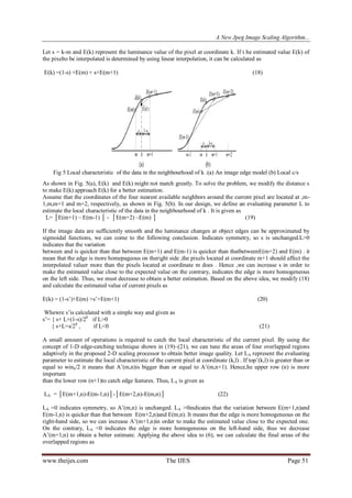
E. Area Tuner
AT is used to modify the areas of the four overlapped regions based on the current local edge
information (LA and U _GE provided by EC). Fig. 13 shows the two-stage pipeline architecture of AT. If U_
GE is equal to 1, the upper row (row n) in current pixel window is more important, so A‟(m,n)and A‟(m+1,n)are
modified according to (23). On the contrary, ifU GE is equal to 0, the lower row (row n+1) is more important,
so A‟(m,n+1) and A‟(m+1,n+1) are modified according to (25). Finally, the tuned areas A‟‟(m,n) , A‟‟(m+1,n) ,
A‟‟(m,n+1) and A‟‟(m+1,n+1) are sent to TG.
Fig 9 Architecture of area tuner
F. Target Generator
By weighted averaging the luminance values of four source pixels with tuned-area coverage ratio, TG
implements (1) and (2) to determine the estimated value FT(k,l). Fig. 14 shows the two-stage pipeline
architecture of TG. Four MULT units and three ADD units are used to perform (1). Since the value of Asum is
equal to the power of 2, the division operation in (2) can be implemented by the shifter easily.
Fig 10 Architecture of target generator .
G. Controller
The controller, realized with a finite-state machine, monitors the data flow and sends proper control
signals to all other components. In the design, AM, AT, and TG require two clock cycles to complete their
functions, respectively. Both AG and EC need one clock cycle to finish their tasks, and they work in parallel
because no data dependency between them exists. For each target pixel, seven clock cycles are needed to output
the estimated value FT(k,l).
V. SIMULATION RESULTS
To evaluate the performance of our image-scaling algorithm, we use 6 gray-scale test images , shown
in. For each single test image, we reduce/enlarge the original image by using the well-known bilinear method,
and then employ various approaches to scale up/down the bilinear-scaled image back to the size of the original
test image. Thus, we can compare the image quality of the reconstructed images for various scaling methods.
Three well-known scaling methods, nearest neighbour (NN) , bilinear (BL) [6], and bicubic (BC) [9], two area-
pixel scaling methods, Win (winscale in [7]) and M Win (the modified winscale in [8]), and our method are used
for comparison in terms of computational complexity, objectivetesting (quantitative evaluation), and subjective
testing (visualquality), respectively. To reduce hardware cost, we adopt the low-cost technique suitable for VLSI
implementation to perform area-pixel scaling.

10. A New Jpeg Image Scaling Algorithm...
www.theijes.com The IJES Page 55
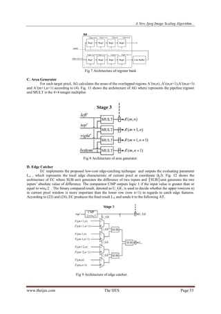
Table I shows the computing time (in the unit of second) of enlarging image “Lena” for the two
processors. Obviously, our method requires less computing time than [7]–[9], and BC needs much longer time
due to extensive computations.To explore the performance of quantitative evaluation for image enlargement and
reduction, first we scale the some test images to the different size of by using the bilinear method. Then, we
scale up/down these images back to the original size and show the results of peak signal-to-noise ratio (PSNR)
in Tables II, III, and IV, respectively. Here, the output images of our scaling method are generated by the
proposed VLSI circuit after post-layout transistor-level simulation. Simulation results show that our design
achieves better quantitative quality than the previous low-complexity scaling methods [5]–[8]. However, the
exact degree of improvement is dependent on the content of different images processed
The proposed VLSI architecture of the proposed design was implemented by using Verilog HDL.We
used SYNOPSYS Design Vision to synthesize the design with TSMC‟s 0.18- m cell library. The layout for the
design was generated with SYNOPSYS Astro (for auto placement and routing), and verified by MENTOR
GRAPHIC Calibre (for DRC and LVS checks), respectively.Modelsim was used for post-layout transistor-level
simulation. Finally, SYNOPSYS Prime Power was employed to measure the total power consumption.
Synthesis results show that the scaling processor contains 10.4-K gate counts and its core size is about 532 521
m . It works with a clock period of 5 ns .
WIN M_WIN Bicubic OUR
Line Buffer 1 1 6 1
Area 29k gate NA 890CLBs 10.4K gate
counts
Max Frquency 65 MHz 55 MHz 100MHz 200MHz
Computation Time 4.74ms 5.60ms 3.50ms 1.54ms
Features of some scaling methods
Area method input image (64 Bit
Area method Scale up image (128 Bit

11. A New Jpeg Image Scaling Algorithm...
www.theijes.com The IJES Page 56
VI. CONCLUSION
A low-cost image scaling processor is proposed in this paper. The experimental results demonstrate
that our design achieves better performances in both objective and subjective image quality than other low-
complexity scaling methods. Furthermore, an efficient VLSI architecture for the proposed method is presented.
In our simulation, it operates with a clock period of 5 ns and achieves a processing rate of 200
megapixels/second.The architecture works with monochromatic images, but it can be extended for working with
RGB color images easily.
REFERENCES
[1] R. C. Gonzalez and R. E.Woods, Digital Image Processing. Reading, MA: Addison-Wesley, 1992.
[2] W. K. Pratt, Digital Image Processing. New York: Wiley-Interscience, 1991.
[3] T. M. Lehmann, C. Gonner, and K. Spitzer, “Survey: Interpolation methods in medical image processing,” IEEE Trans. Med.
Imag., vol. 18, no. 11, pp. 1049–1075, Nov. 1999.
[4] C.Weerasnghe, M. Nilsson, S. Lichman, and I. Kharitonenko, “Digital
zoom camera with image sharpening and suppression,” IEEE Trans. Consumer Electron., vol. 50, no. 3, pp. 777–786, Aug. 2004.
[5] S. Fifman, “Digital rectification of ERTS multispectral imagery,” in
Proc. Significant Results Obtained from Earth Resources Technology Satellite-1, 1973, vol. 1, pp. 1131–1142.
[6] J. A. Parker, R. V. Kenyon, and D. E. Troxel, “Comparison of interpolation
methods for image resampling,” IEEE Trans. Med. Imag., vol. MI-2, no. 3, pp. 31–39, Sep. 1983.
[7] C. Kim, S. M. Seong, J. A. Lee, and L. S. Kim, “Winscale: An image scaling algorithm using an area pixel model,” IEEE Trans.
Circuits Syst. Video Technol., vol. 13, no. 6, pp. 549–553, Jun. 2003.
[8] I. Andreadis and A. Amanatiadis, “Digital image scaling,” in Proc. IEEE Instrum. Meas. Technol. Conf.,May 2005, vol. 3, pp.
2028–2032.
[9] H. S. Hou and H. C. Andrews, “Cubic splines for image interpolation and digital filtering,” IEEE Trans. Acoust. Speech Signal
Process., vol. ASSP-26, no. 6, pp. 508–517, Dec. 1978.
[10] J. K. Han and S. U. Baek, “Parametric cubic convolution scalar for enlargement
and reduction of image,” IEEE Trans. Consumer Electron., vol. 46, no. 2, pp. 247–256, May 2000.
[11] L. J.Wang, W. S. Hsieh, and T. K. Truong, “A fast computation of 2-D
cubic-spline interpolation,” IEEE Signal Process. Lett., vol. 11, no. 9, pp. 768–771, Sep. 2004.
[12] H. A. Aly and E. Dubois, “Image up-sampling using total- variation regularization with a new observation model,” IEEE Trans.
Image Process., vol. 14, no. 10, pp. 1647–1659, Oct. 2005.
[13] T. Feng, W. L. Xie, and L. X. Yang, “An architecture and implementation of image scaling conversion,” in Proc. IEEE Int. Conf.
Appl. Specific Integr. Circuits, 2001, pp. 409–410.
[14] M. A. Nuno-Maganda and M. O. Arias-Estrada, “Real-time FPGAbased
architecture for bicubic interpolation: An application for digital image scaling,” in Proc. IEEE Int. Conf. Reconfigurable
Computing FPGAs, 2005, pp. 8–11.
[15] G. Ramponi, “Warped distance for space-variant linear image interpolation,”
IEEE Trans. Image Process., vol. 8, no. 5, pp. 629–639, May