Exponential lindley additive failure rate model

IJRET: International Journal of Research in Engineering and Technology eISSN: 2319-1163 | pISSN: 2321-7308
_______________________________________________________________________________________
Volume: 04 Issue: 10 | OCT -2015, Available @ http://www.ijret.org 217
EXPONENTIAL-LINDLEYADDITIVE FAILURE RATE MODEL
K.Rosaiah
1
, P.Lakshmi Sravani
2
, K.Kalyani
3
, D.C.U.Siva Kumar
4
1
Department of Statistics, Acharya Nagarjuna University, Guntur – 522 510, India.
2Department of Mathematics & Statistics, K.B.N. College (Autonomous), Vijayawada – 520001, India.
3 Research Fellows (UGC), Department of Statistics, Acharya Nagarjuna University, Guntur – 522510, India.
rosaiah1959@gmail.com
Abstract:
A combination of exponential and Lindley failure rate model is considered and named it as exponential-Lindley
additive failure rate model. In this paper, we studied the distributional properties, central and non-central moments,
estimation of parameters, testing of hypothesis and the power of likelihood ratio criterion about the proposed model.
Key words: Exponential distribution, Lindley distribution, ML estimation, Likelihood ratio type criterion.
---------------------------------------------------------------------***---------------------------------------------------------------------
1. INTRODUCTION
Normal distribution and exponential distribution are the
basic models exemplified in a number of theoretical results
in the theory of distributions. Particularly, exponential
distribution is an invariable example for a number of
theoretical concepts in reliability studies. It is characterized
as constant failure rate (CFR) model also. In case of
necessity for an increasing failure rate (IFR) model
ordinarily the choice falls on Weibull model with shape
parameter more than 1 (>1), in particular taken as 2. Similar
in shape, with common characteristics of Weibull, we have
Lindley distribution as another IFR model. Lindley
distribution has its own prominence as a life testing model.
In this paper, we propose to combine an exponential (CFR)
model and a Lindley (IFR) model through their hazard
functions to get two component series system reliability,
which is given as follows:
1 2
0
[ ( ) ( )]
( )
x
h x h x dx
R x e
 
 (1)
where 1
( )h x and 2
( )h x are respectively, the hazard functions
of exponential and Lindley distributions.
One such situation is the popular linear failure rate
distribution [LFRD]. In that model h1(x) is taken as a
constant failure rate model and h2(x) is taken as an
increasing failure rate (IFR) model with specific choices of
exponential for h1(x) and Weibull with shape 2 for h2(x).
The failure density, the cumulative distribution function, the
reliability function and the failure rate of LFRD model are
respectively given by





 
 2
x
2
xexp)x(),;x(f
2
( ; , ) 1 exp 0, , 0
2
F x x x x

     
      
 
2
( ) ( ; , ) 1 F( ; , ) exp
2
R x F x x x x

    
 
      
 
x),;x(h 
A number of researchers made an extensive study on LFRD
model. Some works in this regard are Bain (1974),
Balakrishnan and Malik (1986), Ananda Sen and
Bhattacharya (1995), Mohie El-Din et al. (1997), Ghitany
and Kotz (2007), ABD EL –Baset A.Ahmad (2008),
Mahmoud and Al-Nagar (2009).
Kantam and Priya (2011) considered an additive life testing
model combining a CFR and DFR model with DFR
generated from a Weibull model of shape parameter < 1.
Srinivasarao et al. (2013a) studied the properties, estimation
and testing of linear failure rate model with exponential and
half – logistic distribution. Srinivasarao et al. (2013b) have
discussed the distributional properties, estimation of
parameters and testing of hypothesis for additive failure rate
model combining exponential and gamma distributions.
Rosaiah et al. (2014) studied the estimation of parameters,
testing of linear failure rate with exponential and modified
Weibull distribution. Srinivas (2015) considered an additive
failure rate model combining exponential and generalized
half logistic distributions.
The probability density function (PDF), cumulative
distribution function (CDF) and hazard function (HF) of the
exponential distribution with scale parameter λ are
respectively given by
1( ; ) ; 0, 0x
f x e x
  
  
1( ; ) 1 ; 0, 0x
F x e x
 
   
1 ( ; )h x  
The Lindley distribution was originally proposed by Lindley
(1958) in the context of Bayesian statistics, a counter
example of fudicial statistics. The PDF, CDF and HF of the
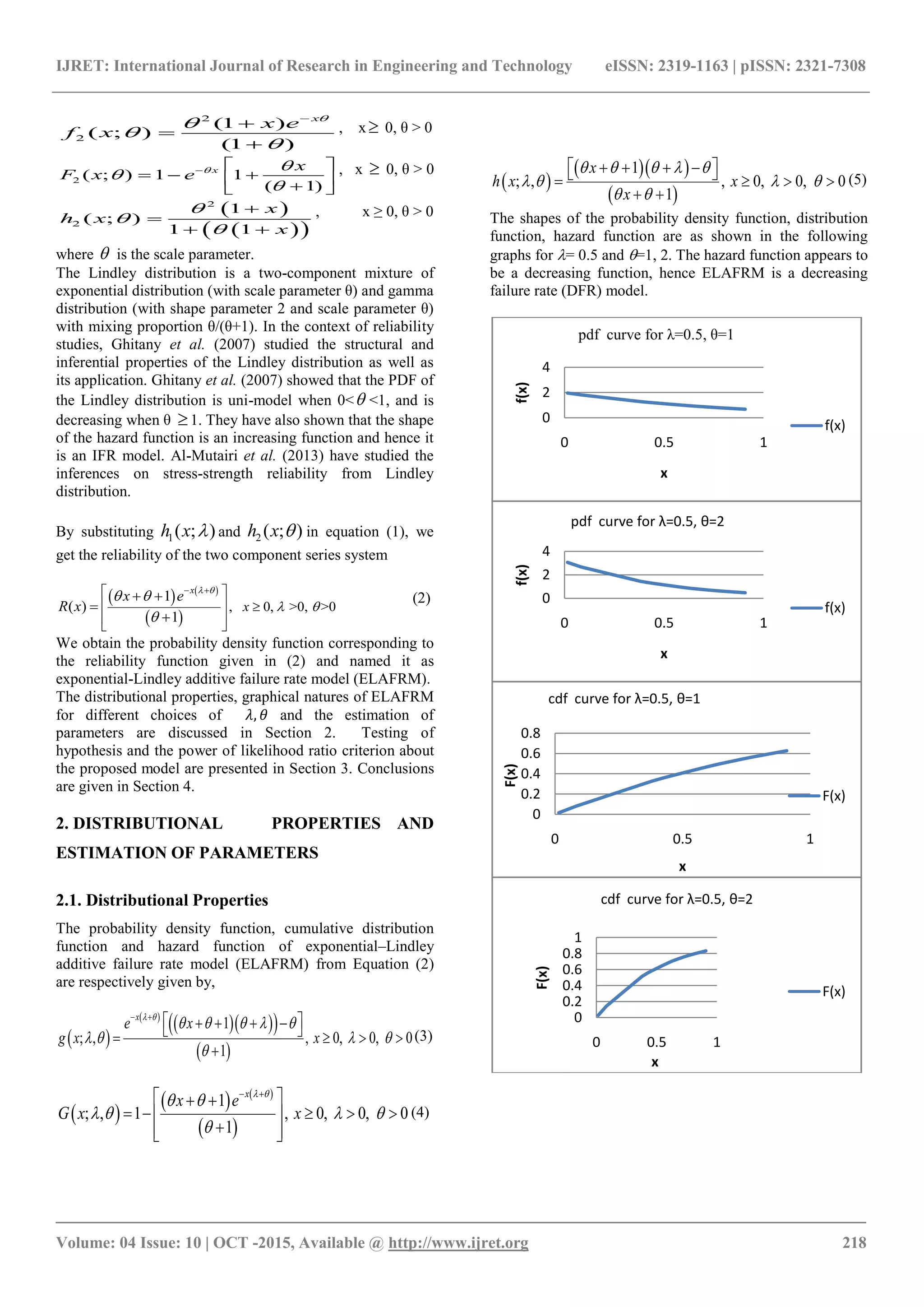
Lindley distribution are respectively given by

_______________________________________________________________________________________
2
2
(1 )
( ; )
(1 )
x
x e
f x








, x  0, θ > 0
2 ( ; ) 1 1
( 1)
x x
F x e  


  
    
, x  0, θ > 0
 
  
2
2
1
( ; )
1 1
x
h x
x





 
, x ≥ 0, θ > 0
where  is the scale parameter.
The Lindley distribution is a two-component mixture of
exponential distribution (with scale parameter θ) and gamma
distribution (with shape parameter 2 and scale parameter θ)
with mixing proportion θ/(θ+1). In the context of reliability
studies, Ghitany et al. (2007) studied the structural and
inferential properties of the Lindley distribution as well as
its application. Ghitany et al. (2007) showed that the PDF of
the Lindley distribution is uni-model when 0< <1, and is
decreasing when θ 1. They have also shown that the shape
of the hazard function is an increasing function and hence it
is an IFR model. Al-Mutairi et al. (2013) have studied the
inferences on stress-strength reliability from Lindley
distribution.
By substituting 1( ; )h x  and 2 ( ; )h x  in equation (1), we
get the reliability of the two component series system
   
 
, 0, >0, >0
1
( )
1
x
x
x e
R x
 
 
 

  
  
 
 
 


(2)
We obtain the probability density function corresponding to
the reliability function given in (2) and named it as
exponential-Lindley additive failure rate model (ELAFRM).
The distributional properties, graphical natures of ELAFRM
for different choices of 𝜆, 𝜃 and the estimation of
parameters are discussed in Section 2. Testing of
hypothesis and the power of likelihood ratio criterion about
the proposed model are presented in Section 3. Conclusions
are given in Section 4.
2. DISTRIBUTIONAL PROPERTIES AND
ESTIMATION OF PARAMETERS
2.1. Distributional Properties
The probability density function, cumulative distribution
function and hazard function of exponential–Lindley
additive failure rate model (ELAFRM) from Equation (2)
are respectively given by,
 
 
   
 
1
; , , 0, 0, 0
1
x
e x
g x x
 
    
   

 
        

(3)
 
   
 
1
; , 1 , 0, 0, 0
1
x
x e
G x x
 
 
   

 
  
     
  
(4)
 
  
 
1
; , , 0, 0, 0
1
x
h x x
x
    
   
 
        
 
(5)
The shapes of the probability density function, distribution
function, hazard function are as shown in the following
graphs for = 0.5 and =1, 2. The hazard function appears to
be a decreasing function, hence ELAFRM is a decreasing
failure rate (DFR) model.
0
2
4
0 0.5 1
f(x)
x
pdf curve for λ=0.5, θ=1
f(x)
0
2
4
0 0.5 1
f(x)
x
pdf curve for λ=0.5, θ=2
f(x)
0
0.2
0.4
0.6
0.8
0 0.5 1
F(x)
x
cdf curve for λ=0.5, θ=1
F(x)
0
0.2
0.4
0.6
0.8
1
0 0.5 1
F(x)
x
cdf curve for λ=0.5, θ=2
F(x)

_______________________________________________________________________________________
Central and non-central moments of ELAFRM are as
follows:
Non–Central moments:
 
 
 
 
1 1
1 22 3
1 ( 2) 2 1 2 ( 3)
,
1 ( ) 1 ( )
       
 
     
     
 
   
 
 
 
 
1 1
3 44 5
6 1 6 ( 4) 24 1 24 ( 5)
,
1 ( ) 1 ( )
       
 
     
     
 
   
CENTRAL MOMENTS:
 
1 2
( 1) ( 2)
( 1)( )
   

  
  

 
 
2
2 3
( 1) ( 2)1
2 ( 1) 2 ( 3)
( 1)( ) ( 1)( )
   
    
     
    
       
       
 
    
3
2 2
3 4
6 ( 1) 6 ( 4)
2 ( 1) 2 ( 3) ( 1) ( 2) ( 1) ( 2)
3 2
( 1)( ) ( 1) ( )
1
( 1)( )
   
           
     

  
   
  
           
             

 
4 5 4 2
2
3 2
( 1) ( 2)24 ( 1) 24 ( 5) 6 ( 1) 6 ( 4)
4
( 1)( ) ( 1)( ) ( 1)( )
( 1) ( 2) ( 12 ( 1) 2 ( 3)
6 3
( 1)( ) ( 1)( )
          
        
        
     
         
         
       
     
       
  
     
     

   
4
2
) ( 2)
( 1)( )
 
  
    
 
 
 
 
2.2. Maximum Likelihood Estimation (MLE)
Let 1 2, ,..., nx x x be a random sample of size n drawn from ELAFRM with density function g(x;λ, θ), then the likelihood function
of  1 2, ,..., nx x x is given by
 
 
   
 1 1
1
; ,
1
in
i
i
i
xn
i
x
L g x
e
L
 
    
 

 

    
 
 
 
 
 
1.8
1.9
2
2.1
0 0.5 1
h(x)
x
hazard function for λ=0.5, θ=1
h(x)
2.9
3
3.1
3.2
0 0.5 1
h(x)
x
hazard function for λ=0.5, θ=2
h(x)

_______________________________________________________________________________________
        
1 1
log log 1 log 1
n n
i i
i i
L x x n       
 
           
The MLE’s 𝜆, 𝜃 of  and θ can be obtained by simultaneously solving the following ML equations,
log
0
L




 
   1 1
1
0
1
n n
i
i
i i i
x
x
x
 
       
 
 
   
   
 
log
0
L




     
     1 1
1 1 1
0
11
n n
i i
i
i i i
x x n
x
x
   
     
 
 
  
   
     
    
   
 
The asymptotic variances and covariance of the estimators of the parameters are obtained using the following elements of the
information matrix
 
   
22
11 22
1
1log
1
n
i
i
i
xL
I E E
x
 
     
  
                        

  
   
2
12 21 2
1
1 2log
1
n
i i
i
i
x xL
I I E E
x
  
      
  
                           

     
     
     
2
22 2
2
2 2
1
log
1 1 1
1 2 2
11
i i
n i i
i
i
L
I E
x x
x x
n
E
x

   
    
    
  
   
    
  
   
                             
  
  
   
      
    
   
   

The estimated asymptotic variance-covariance matrix of the MLEs is given by
  22 122 1
11 22 12
21 11
ˆ ˆ
ˆ ˆ ˆ, =[ ]
ˆ ˆ
I I
D I I I
I I
  
 
  
  
 
2 2 2
11 22 12 212 2
,, ,
log log logˆ ˆ ˆ ˆ= , = ,
L L L
where I E I E I I E
          
       
       
        
       
    
3. LIKELIHOOD RATIO TYPE CRITERION AND CRITICAL VALUES
Let us designate our proposed ELAFRM as null population
say P0 and exponential distribution as alternate population
say P1. We propose a null hypothesis H0 : “A given sample
belongs to the population P0” against an alternative
hypothesis H1 : “The sample belongs to population P1”.
Let L1, L0 respectively stand for the likelihood functions of
the sample with population P1 and P0. Both L1 and L0
contains the respective parameters of the populations. The
given sample is used to get the parameters of P1, P0 , so that
for the given sample, the value of
𝐿1
𝐿0
is now
estimated. If H0 is true,
𝐿1
𝐿0
must be small, therefore for
accepting H0 with a given degree of confidence,
𝐿1
𝐿0
is
compared with a critical value with the help of the
percentiles in the sampling distribution of
𝐿1
𝐿0
.
We have seen in Section 2.2, how to get the estimates of
parameters. But the sampling distribution of
𝐿1
𝐿0
is not
analytical, we therefore resorted to the empirical sampling
distribution through simulation. We have generated 3000
random samples of size n=5(1)10 from the population P0
with various parameter combinations and obtain the values
of L1, L0 along with the estimates of respective parameters
for each sample.
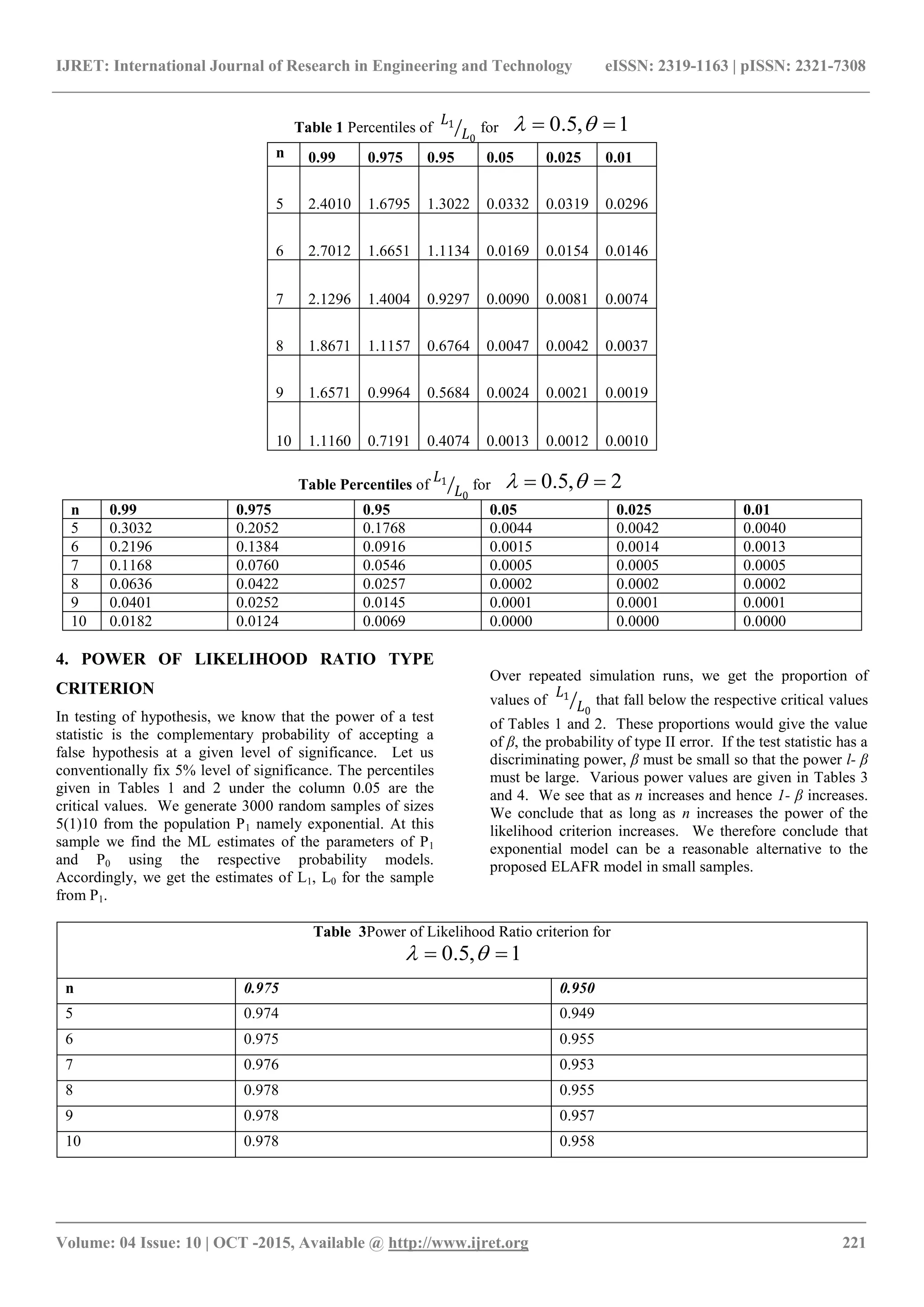
The percentiles of
𝐿1
𝐿0
at various probabilities are
computed and are given in Tables 1 and 2.

_______________________________________________________________________________________
Table 1 Percentiles of
𝐿1
𝐿0
for 0.5, 1  
n 0.99 0.975 0.95 0.05 0.025 0.01
5 2.4010 1.6795 1.3022 0.0332 0.0319 0.0296
6 2.7012 1.6651 1.1134 0.0169 0.0154 0.0146
7 2.1296 1.4004 0.9297 0.0090 0.0081 0.0074
8 1.8671 1.1157 0.6764 0.0047 0.0042 0.0037
9 1.6571 0.9964 0.5684 0.0024 0.0021 0.0019
10 1.1160 0.7191 0.4074 0.0013 0.0012 0.0010
Table Percentiles of
𝐿1
𝐿0
for 0.5, 2  
n 0.99 0.975 0.95 0.05 0.025 0.01
5 0.3032 0.2052 0.1768 0.0044 0.0042 0.0040
6 0.2196 0.1384 0.0916 0.0015 0.0014 0.0013
7 0.1168 0.0760 0.0546 0.0005 0.0005 0.0005
8 0.0636 0.0422 0.0257 0.0002 0.0002 0.0002
9 0.0401 0.0252 0.0145 0.0001 0.0001 0.0001
10 0.0182 0.0124 0.0069 0.0000 0.0000 0.0000
4. POWER OF LIKELIHOOD RATIO TYPE
CRITERION
In testing of hypothesis, we know that the power of a test
statistic is the complementary probability of accepting a
false hypothesis at a given level of significance. Let us
conventionally fix 5% level of significance. The percentiles
given in Tables 1 and 2 under the column 0.05 are the
critical values. We generate 3000 random samples of sizes
5(1)10 from the population P1 namely exponential. At this
sample we find the ML estimates of the parameters of P1
and P0 using the respective probability models.
Accordingly, we get the estimates of L1, L0 for the sample
from P1.
Over repeated simulation runs, we get the proportion of
values of
𝐿1
𝐿0
that fall below the respective critical values
of Tables 1 and 2. These proportions would give the value
of β, the probability of type II error. If the test statistic has a
discriminating power, β must be small so that the power l- β
must be large. Various power values are given in Tables 3
and 4. We see that as n increases and hence 1- β increases.
We conclude that as long as n increases the power of the
likelihood criterion increases. We therefore conclude that
exponential model can be a reasonable alternative to the
proposed ELAFR model in small samples.
Table 3Power of Likelihood Ratio criterion for
0.5, 1  
n 0.975 0.950
5 0.974 0.949
6 0.975 0.955
7 0.976 0.953
8 0.978 0.955
9 0.978 0.957
10 0.978 0.958

_______________________________________________________________________________________
Table 4Power of Likelihood Ratio criterion for
0.5, 2  
n 0.975 0.950
5 0.969 0.968
6 0.978 0.977
7 0.983 0.980
8 0.984 0.983
9 0.991 0.987
10 0.991 0.988
5. CONCLUSIONS
Exponential and Lindley failure rate models are considered
for reliability studies and are named as exponential-Lindley
additive failure rate model. The distributional properties,
estimation of parameters, testing of hypothesis and the
power of likelihood ratio criterion about the proposed model
are discussed and the results are presented.
REFERENCES
[1]. ABD EL – Baset A. Ahmad. (2008). “Single and
product moments of generalized ordered statistics
from linear exponential distributions”,
Communications in Statistics – Theory and Methods,
37, 1162 - 1172.
[2]. Al-Mutairi, D.K., Ghitany, M.E., Kundu, D. (2013).
Inference on stress-strength reliability from Lindley
distribution, Communications in Statistics - Theory
and Methods, 42: 1443-1463.
[3]. Ammar M. Sarhan and Debasis Kundu (2009).
“Generalized linear failure rate distribution”,
Communications in Statistics – Theory and Methods,
38 (5), 642 – 660.
[4]. Ananda Sen and Bhattacharyya, G.K. (1995).
“Inference procedures for the linear failure rate
model”, Journal of Statistical Planning and Inference,
46, 59-76.
[5]. Bain, L.J. (1974). “Analysis for the linear failure rate
life-testing distribution”, Technometrics, 16 (4), 551
– 559.
[6]. Balakrishnan, N. and Malik, H.J. (1986). “Order
statiscs from the linear-exponential distribution, part
I : Increasing hazard rate case”, Communications in
Statistics, Theory and Methods, 15, 179 – 203.
[7]. Ghitany, M. E. and Samual Kotz. (2007). “Reliability
properties of extended linear failure rate
distributions”, Probability in the Engineering and
Informational Sciences, 21, 441 – 450.
[8]. Kantam, R.R.L. and Priya, M.Ch. (2011). “An
additive life testing model”, Paper presented at
Conference on statistical Techniques in Life-Testing,
Reliability, Sampling theory and Quality Control,
Banaras Hindu University, Varanasi, Jan 4 -7.
[9]. Lindley, D.V, (1958). “Fiducial distributions and
Bayes’ theorem”, Journal of the Royal Statistical
Society 20(1), 102-107.
[10]. Mahmoud, M.A.W. and Al-Nagar H.SH. (2009). “On
generalized order statistics from linear exponential
distribution and its characterization”, Stat Papers, 50,
407 – 418.
[11]. M.M. Mohie El-Din, M.A.W. Mahmoud, S.E. Abu-
Youseff, K.S. Sultan (1997). “Ordered statistics
from the doubly truncated linear exponential
distribution and its characterization”,
Communications in Statistics – Simulation and
Computation, 26 (1), 281 – 290.
[12]. Rosaiah, K., Srinivasa Rao, B., Nargis Fathima
Mohamad and C. U. SivaKumar, D. (2014).
Exponential – Modified Weibull additive failure rate
model, International
[13]. Journal of Technology and Research Advances, Issue
VI, pp 1-10.
[14]. Srinivasa Rao, B., Nagendram, S. and Rosaiah, K.
(2013a). Exponential – Half logistic additive failure
rate model, International Journal of Scientific and
Research publications, 3(5), 1-10.
[15]. Srinivasa Rao, B., Sridhar Babu, M. and Rosaiah, K.
(2013b). Exponential – gamma additive failure rate
model, Journal of Safety Engineering, 2(2A), 1-6.
[16]. Srinivas , I, L. (2015). “Exponential- generalized half
logistic Additive failure rate model: an inferential
study,Un published M.phil dissertation, Acharya
Nagarjuna University, India.

Exponential lindley additive failure rate model

More Related Content

What's hot

Viewers also liked

Similar to Exponential lindley additive failure rate model

More from eSAT Journals

Recently uploaded

Exponential lindley additive failure rate model