Downloaded 12 times
![Mathematical Theory and Modeling
ISSN 2224-5804 (Paper) ISSN 2225-0522 (Online)
Vol.3, No.13, 2013
www.iiste.org
A new generalized Lindley distribution
Ibrahim Elbatal1 Faton Merovci2* M. Elgarhy3
1.
Institute of Statistical Studies and Research, Departmentof Mathematical Statistics, Cairo University.
2.
3.
Department of Mathematics, University of Prishtina "Hasan Prishtina" Republic of Kosovo
Institute of Statistical Studies and Research, Departmentof Mathematical Statistics, Cairo
1
University.
E-mail: i_elbatal@staff.cu.edu.eg
2
* E-mail of the corresponding author: fmerovci@yahoo.com
3
E-mail: m_elgarhy85@yahoo.com
Abstract
In this paper, we present a new class of distributions called New Generalized Lindley
Distribution(NGLD). This class of distributions contains several distributions such as gamma, exponential
and Lindley as special cases. The hazard function, reverse hazard function, moments and moment
generating function and inequality measures are are obtained. Moreover, we discuss the maximum
likelihood estimation of this distribution. The usefulness of the new model is illustrated by means of two
real data sets. We hope that the new distribution proposed here will serve as an alternative model to other
models available in the literature for modelling positive real data in many areas.
Keywords: Generalized Lindley Distribution; Gamma distribution, Maximum likelihood estimation;
Moment generating function.
1 Introduction and Motivation
In many applied sciences such as medicine, engineering and finance, amongst others, modeling and
analyzing lifetime data are crucial. Several lifetime distributions have been used to model such kinds of data. For
instance, the exponential, Weibull, gamma, Rayleigh distributions and their generalizations ( see, e.g., Gupta and
Kundu, [10]). Each distribution has its own characteristics due specifically to the shape of the failure rate
function which may be only monotonically decreasing or increasing or constant in its behavior, as well as nonmonotone, being bathtub shaped or even unimodal. Here we consider the Lindley distribution which was
introduced by Lindley [13]. Let the life time random variable X has a Lindley distribution with parameter q ,
the probability density function (pdf) of X is given by
q2
g ( x,q ) =
(1 + x)e -q x ; x > 0,q > 0,
q +1
(1)
It can be seen that this distribution is a mixture of exponential (q ) and gamma (2,q ) distributions. The
corresponding cumulative distribution function (cdf) of LD is obtained as
G( x,q ) = 1 -
q + 1 + qx -q x
e , x > 0,q > 0,
q +1
(2)
where q is scale parameter. The Lindley distribution is important for studying stress–strength reliability
modeling. Besides, some researchers have proposed new classes of distributions based on modifications of the
Lindley distribution, including also their properties. The main idea is always directed by embedding former
distributions to more flexible structures. Sankaran [16] introduced the discrete Poisson–Lindley distribution by
combining the Poisson and Lindley distributions. Ghitany et al. [5] have discussed various properties of this
distribution and showed that in many ways Equation (1) provides a better model for some applications than the
exponential distribution. A discrete version of this distribution has been suggested by Deniz and Ojeda [3] having
its applications in count data related to insurance. Ghitany et al. [7, 8] obtained size-biased and zero-truncated
version of Poisson- Lindley distribution and discussed their various properties and applications. Ghitany and AlMutairi [6] discussed as various estimation methods for the discrete Poisson- Lindley distribution. Bakouch et al.
[1] obtained an extended Lindley distribution and discussed its various properties and applications. Mazucheli
and Achcar [14] discussed the applications of Lindley distribution to competing risks lifetime data. Rama and
30](https://image.slidesharecdn.com/anewgeneralizedlindleydistribution-131202193225-phpapp01/75/A-new-generalized-lindley-distribution-1-2048.jpg)
![Mathematical Theory and Modeling
ISSN 2224-5804 (Paper) ISSN 2225-0522 (Online)
Vol.3, No.13, 2013
www.iiste.org
Mishra [15] studied quasi Lindley distribution. Ghitany et al. [9] developed a two-parameter weighted Lindley
distribution and discussed its applications to survival data. Zakerzadah and Dolati [18] obtained a generalized
Lindley distribution and discussed its various properties and applications.
This paper offers new distribution with three parameter called generalizes the Lindley distribution, this
distribution includes as special cases the ordinary exponential and gamma distributions. The procedure used here
is based on certain mixtures of the gamma distributions. The study examines various properties of the new model.
The rest of the paper is organized as follows: Various statistical properties includes moment, generating function
and inequality measures of the NGL distribution are explored in Section 2. The distribution of the order statistics
is expressed in Section 3. We provide the regression based method of least squares and weighted least squares
estimators in Section 4. Maximum likelihood estimates of the parameters index to the distribution are discussed
in Section 5. Section 6 provides applications to real data sets. Section 7 ends with some conclusions
2 Statistical Properties and Reliability Measures
In this section, we investigate the basic statistical properties, in particular,
generating function and inequality measures for the
rth moment, moment
NGL distribution.
2.1 Density survival and failure rate functions
The new generalized Lindley distribution is denoted as NGLD(a , b ,q ) . This generalized model is
obtained from a mixture of the gamma (a ,q ) and gamma ( b ,q ) distributions as follows:
f ( x,q , a , b ) = pf1 ( x, a ,q ) + (1 - p) f 2 ( x, b ,q )
=
1 éq a +1 x a -1 q b x b -1 ù -q x
+
ê
úe ;a ,q > 0, x > 0. (3)
G( b ) û
1 + q ë G(a )
where
p=
q
1+q
,
f1 ( x, a ,q ) =
q (qx)a -1 -q x
q (qx) b -1 -q x
e and f 2 ( x, b ,q ) =
e .
G(a )
G( b )
The corresponding cumulative distribution function (cdf) of generalized Lindley is given by
F ( x,q , a , b ) =
1 éqg (a ,qx) g ( b ,qx) ù
+
, (4)
1 + q ê G(a )
G( b ) ú
ë
û
where
t
g ( s, t ) = òx s -1e - x dx
0
is called lower incomplete gamma. Also the upper incomplete gamma is given by
¥
G(a , t ) = òxa -1e - x dx
t
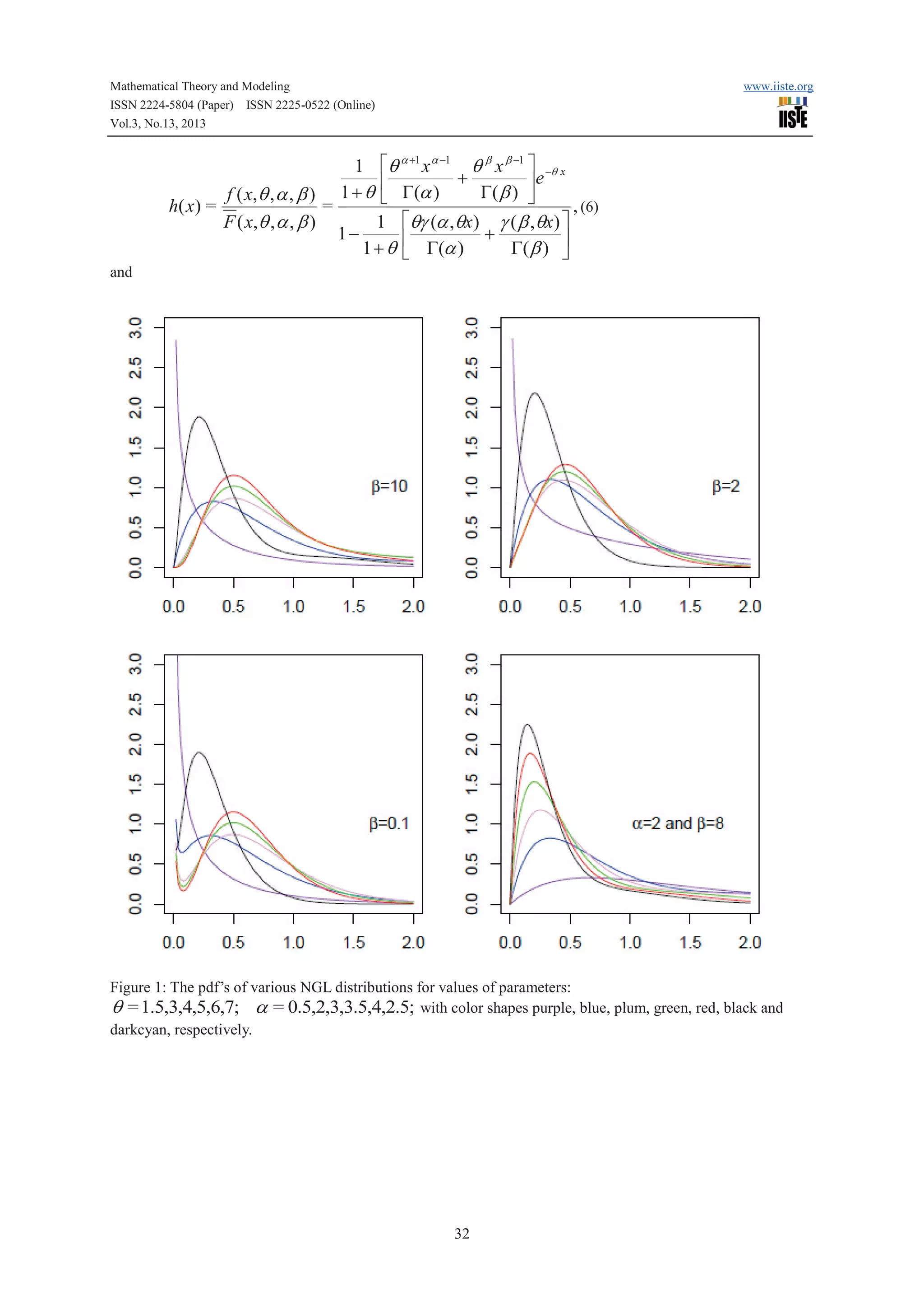
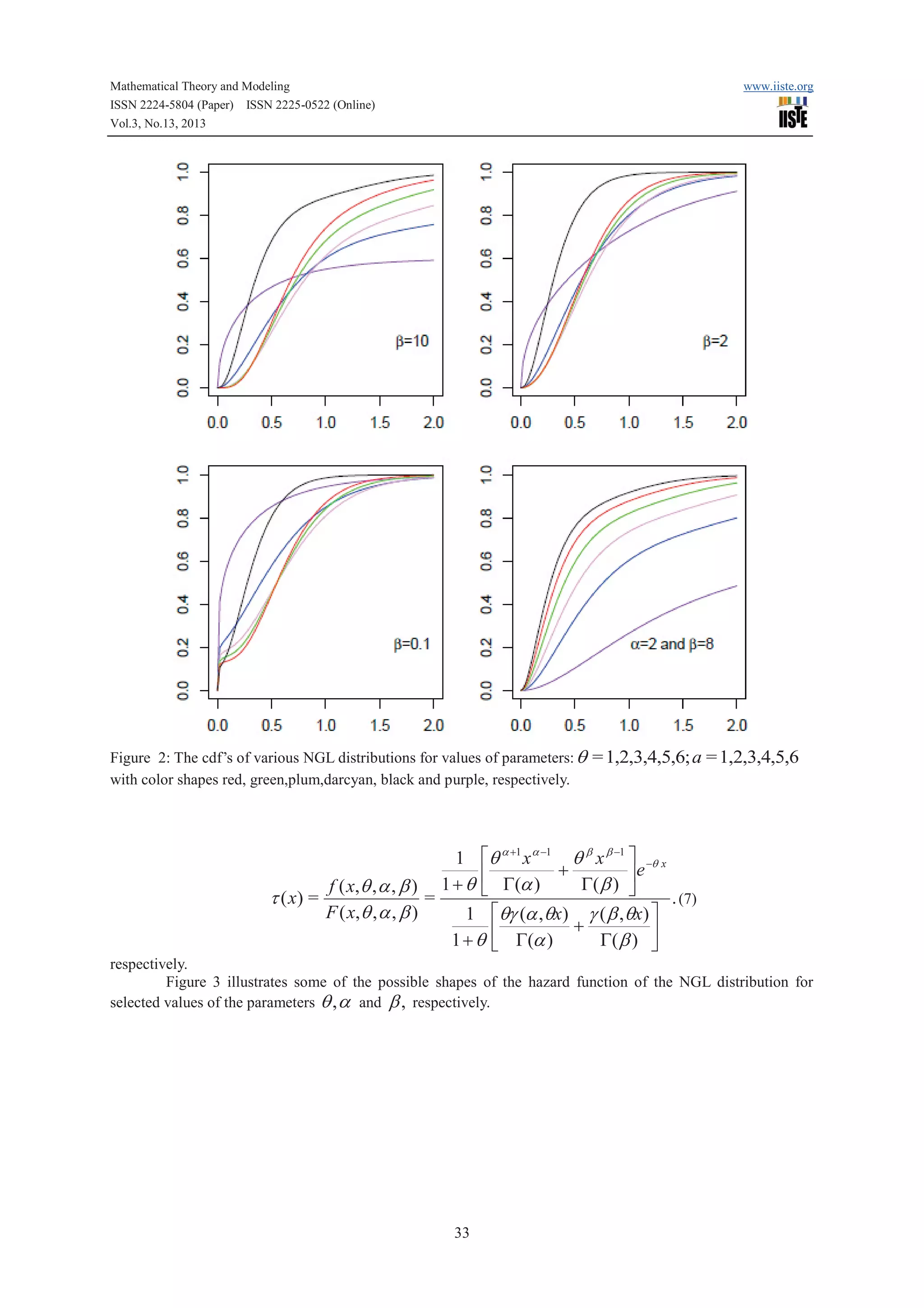
For more details about the definition of incomplete gamma, see Wall [20]. Figures 0 and 1 illustrates some of
the possible shapes of the pdf and cdf of the NGL distribution for selected values of the parameters q , a and
b,
respectively.
The survival function associated with (4) is given by
F ( x,q , a , b ) = 1 - F ( x,q , a , b ) = 1 -
1 éqg (a ,qx) g ( b ,qx) ù
, (5)
+
1 + q ê G(a )
G( b ) ú
ë
û
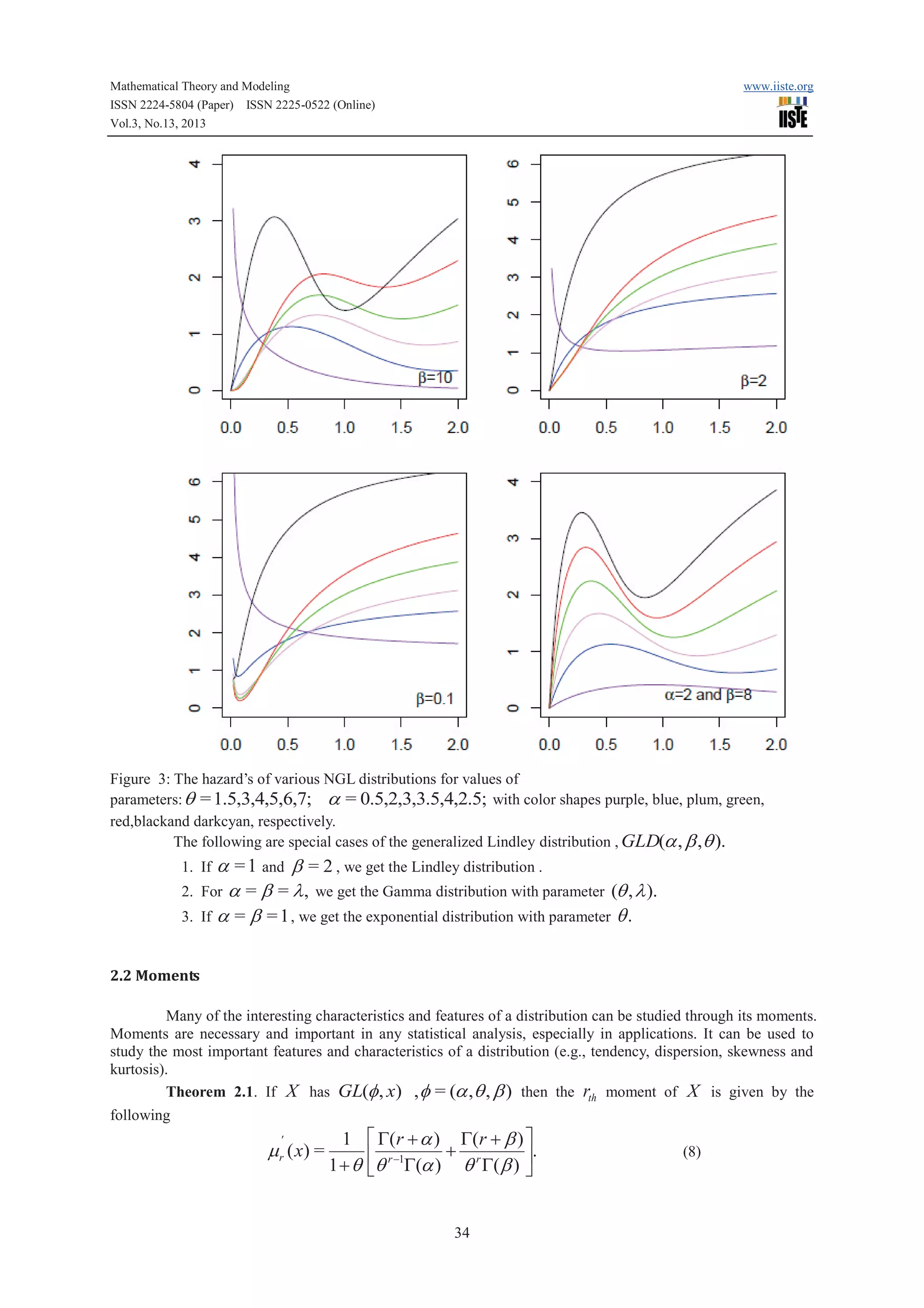
From (??), (4) and (5), the failure (or hazard) rate function (hf) and reverse hazard functions (rhf) of generalized
Lindley distribution are given by
31](https://image.slidesharecdn.com/anewgeneralizedlindleydistribution-131202193225-phpapp01/75/A-new-generalized-lindley-distribution-2-2048.jpg)
![Mathematical Theory and Modeling
ISSN 2224-5804 (Paper) ISSN 2225-0522 (Online)
Vol.3, No.13, 2013
www.iiste.org
Proof:
Let X be a random variable following the GL distribution with parameters q , a and
Expressions for mathematical expectation,
variance and the rth moment on the origin of X can be obtained using the well-known formula
b
.
¥
'
m r ( x) = E ( X r ) = òx r f ( x, f )dx
0
a +1 ¥
q b ¥ r + b -1 -qx ù
1 éq
x r +a -1e -qx dx +
x
e dx ú
ê
1 + q ë G(a ) ò
G( b ) ò
0
0
û
1 é G( r + a ) G( r + b ) ù
.
=
+
1 + q êq r -1G(a ) q r G( b ) ú
ë
û
=
Which completes the proof .
Based on the first four moments of the
(9)
GL distribution, the measures of skewness A(j ) and kurtosis
k (j ) of the GL distribution can obtained as
A(j ) =
m 3 (q ) - 3m1 (q ) m 2 (q ) + 2m13 (q )
[m
2
(q ) - m (q )
2
1
]
3
2
,
and
k (j ) =
m 4 (q ) - 4m1 (q ) m3 (q ) + 6m12 (q ) m2 (q ) - 3m14 (q )
[m (q ) - m
2
1
2
(q )
]
2
.
2.3 Moment generating function
In this subsection we derived the moment generating function of
Theorem (2.2): If X has
following form
M X (t ) =
GL distribution.
GL distribution, then the moment generating function M X (t ) has the
1 é q a +1
qb ù
+
ú.
ê
1 + q ë (q - t )a (q - t ) b û
(10)
Proof.
We start with the well known definition of the moment generating function given by
¥
M X (t ) = E (e ) = òetx f GL ( x, f )dx
tX
0
éq
q b ¥ b -1 -(q -t ) x ù
xa -1e -(q -t ) x dx +
x e
dx ú
ê
G(a ) ò
G( b ) ò
0
0
ë
û
a +1
b
ù
1 é q
q
=
+
ê
a
b ú
1 + q ë (q - t )
(q - t ) û
=
1
1+q
a +1 ¥
Which completes the proof.
In the same way, the characteristic function of the
i = - 1 is the unit imaginary number.
35
(11)
GL distribution becomes j (t ) = M X (it ) where
X](https://image.slidesharecdn.com/anewgeneralizedlindleydistribution-131202193225-phpapp01/75/A-new-generalized-lindley-distribution-6-2048.jpg)
![Mathematical Theory and Modeling
ISSN 2224-5804 (Paper) ISSN 2225-0522 (Online)
Vol.3, No.13, 2013
www.iiste.org
2.4 Inequality Measures
Lorenz and Bonferroni curves are the most widely used inequality measures in income and wealth
distribution (Kleiber, 2004). Zenga curve was presented by Zenga [19]. In this section, we will derive Lorenz,
Bonferroni and Zenga curves for the GL distribution. The Lorenz, Bonferroni and Zenga curves are defined by
t
é g (a + 1,qt ) g ( b + 1,qt ) ù
ê G(a ) + qG( b ) ú
û.
=ë
bù
E( X )
é
êa + q ú
ë
û
òxf ( x)dx
LF ( x) =
0
(12)
t
òxf ( x)dx
BF ( x) =
0
E ( X ) F ( x)
=
LF ( x)
F ( x)
é g (a + 1,qt ) g ( b + 1,qt ) ù
(1 + q ) ê
+
qG( b ) ú
ë G(a )
û,
=
b ù éqg (a ,qx) g ( b ,qx) ù
é
êa + q ú ê G(a ) + G( b ) ú
ûë
ë
û
(13)
m - ( x)
,
m + ( x)
(14)
and
AF ( x) = 1 where
t
m - ( x) =
é g (a + 1,qt ) g ( b + 1,qt ) ù
ê G(a ) + qG( b ) ú
û
=ë
bù
E( X )
é
êa + q ú
û
ë
òxf ( x)dx
0
and
¥
+
m ( x) =
òxf ( x)dx
t
1 - F ( x)
1 é G(a + 1, qt ) G( b + 1, qt ) ù
+
qG( b ) ú
(1 + q ) ê G(a )
ë
û.
=
1 éqg (a ,qx) g ( b ,qx) ù
1+
1 + q ê G(a )
G( b ) ú
ë
û
respectively.
The mean residual life (mrl) function computes the expected remaining survival time of a subject given
survival up to time x . We have already defined the mrl as the expectation of the remaining survival
time given survival up to time x(see Frank Guess and Frank Proschan [4].
3 Distribution of the order statistics
rth order statistic of the GL
distribution, also, the measures of skewness and kurtosis of the distribution of the rth order statistic in a sample
In this section, we derive closed form expressions for the pdfs of the
36](https://image.slidesharecdn.com/anewgeneralizedlindleydistribution-131202193225-phpapp01/75/A-new-generalized-lindley-distribution-7-2048.jpg)
![Mathematical Theory and Modeling
ISSN 2224-5804 (Paper) ISSN 2225-0522 (Online)
Vol.3, No.13, 2013
www.iiste.org
n for different choices of n; r are presented in this section. Let X 1 , X 2 ,..., X n be a simple random
sample from GL distribution with pdf and cdf given by (??) and (4), respectively.
Let X 1 , X 2 ,..., X n denote the order statistics obtained from this sample. We now give the probability
density function of X r:n , say f r:n ( x, f ) and the moments of X r:n , r = 1,2,..., n . Therefore, the measures of
skewness and kurtosis of the distribution of the X r:n are presented. The probability density function of X r:n is
of size
given by
1
[F ( x, f ))]r -1[1 - F ( x,f ))]n-r f ( x,f )) (15)
B(r , n - r + 1)
where f ( x, f )) and F ( x, f )) are the pdf and cdf of the GL distribution given by (3) and (4), respectively,
and B (.,.) is the beta function, since 0 < F ( x, f )) < 1 , for x > 0 , by using the binomial series expansion of
f r:n ( x, F) =
[1 - F ( x,f ))]n-r , given by
j
n-rö
÷[F ( x, f ))] ,
÷
è j ø
ç
[1 - F ( x, f ))]n-r = å(-1) j æ
ç
n-r
j =0
(16)
we have
n-r
æn - rö
r + j -1
(17)
f ( x, f )),
f r:n ( x, f )) = å(-1) j ç
ç j ÷[F ( x, F)]
÷
j =0
è
ø
substituting from (??) and (4) into (17), we can express the k th ordinary moment of the rth order statistics X r:n
k
say E ( X r:n ) as a liner combination of the
kth moments of the GL distribution with different shape parameters.
Therefore, the measures of skewness and kurtosis of the distribution of
X r:n can be calculated.
4 Least Squares and Weighted Least Squares Estimators
GL
In this section we provide the regression based method estimators of the unknown parameters of the
distribution, which was originally suggested by Swain, Venkatraman and Wilson [17] to estimate the
parameters of beta distributions. It can be used some other cases also. Suppose
size
Y1 ,..., Yn is a random sample of
n from a distribution function G(.) and suppose Y(i ) ; i = 1,2,..., n denotes the ordered sample. The
proposed method uses the distribution of G (Y(i ) ) . For a sample of size
n , we have
j
j (n - j + 1)
,V (G(Y( j ) ) ) =
n +1
(n + 1) 2 (n + 2)
j (n - k + 1)
; for j < k ,
andCov(G(Y( j ) ), G(Y( k ) ) ) =
(n + 1) 2 (n + 2)
E (G(Y( j ) ) ) =
see Johnson, Kotz and Balakrishnan [11]. Using the expectations and the variances, two variants of the least
squares methods can be used.
Method 1 (Least Squares Estimators) . Obtain the estimators by minimizing
2
j ö
æ
åç G(Y( j ) - n + 1 ÷ ,
ø
j =1 è
with respect to the unknown parameters. Therefore in case of GL distribution the least squares estimators of
ˆ
ˆ
ˆ
a ,q , and b , say a LSE , q LSE and b LSE respectively, can be obtained by minimizing
n
é 1 éqg (a ,qx ) g ( b ,qx ) ù
j ù
åê1 + q ê G(a )( j ) + G(b )( j ) ú - n + 1ú
j =1 ë
û
ë
û
n
37
2](https://image.slidesharecdn.com/anewgeneralizedlindleydistribution-131202193225-phpapp01/75/A-new-generalized-lindley-distribution-8-2048.jpg)
![Mathematical Theory and Modeling
ISSN 2224-5804 (Paper) ISSN 2225-0522 (Online)
Vol.3, No.13, 2013
www.iiste.org
ˆ
ˆ
ˆ
ˆ
w = 2(l(j; x) - l(j0 ; x)) , where j and j 0 are the MLEs under H1 and H 0 , respectively. The statistic w
2
is asymptotically (as n ® ¥ ) distributed as c k , where k is the length of the parameter vector j of interest.
The LR test rejects
H 0 if w > c k2;g , where c k2;g denotes the upper 100g % quantile of the c k2 distribution.
6 Applications
In this section, we use two real data sets to show that the beta Lindley distribution can be a better model
than one based on the Lindley distribution.
Data set 1: The data set given in Table 1 represents an uncensored data set corresponding to remission
times (in months) of a random sample of 128 bladder cancer patients reported in Lee and Wang [12]:
Table 1: The remission times (in months) of bladder cancer patients
0.08
0.52
2.09
4.98
3.48
6.97
4.87
9.02
6.94
13.29
8.66
0.40
13.11
2.26
23.63
3.57
0.20
5.06
2.23
7.09
0.82
0.62
0.39
0.96
0.19
0.66
0.40
0.26
0.31
0.73
0.51
3.82
10.34
36.66
2.75
11.25
3.02
11.98
4.51
2.07
2.54
5.32
14.83
1.05
4.26
17.14
4.34
19.13
6.54
3.36
3.70
7.32
34.26
2.69
5.41
79.05
5.71
1.76
8.53
6.93
5.17
10.06
0.90
4.23
7.63
1.35
7.93
3.25
12.03
8.65
7.28
14.77
2.69
5.41
17.12
2.87
11.79
4.50
20.28
12.63
9.74
32.15
4.18
7.62
46.12
5.62
18.10
6.25
2.02
22.69
14.76
2.64
5.34
10.75
1.26
7.87
1.46
8.37
3.36
5.49
26.31
3.88
7.59
16.62
2.83
11.64
4.40
12.02
6.76
0.81
5.32
10.66
43.01
4.33
17.36
5.85
2.02
12.07
Data set 2: The following data represent the survival times (in days) of 72 guinea pigs infected with
virulent tubercle bacilli, observed and reported by Bjerkedal [2]. The data are as follows:
0.1, 0.33, 0.44, 0.56, 0.59, 0.72, 0.74, 0.77, 0.92, 0.93, 0.96, 1, 1, 1.02, 1.05, 1.07, 1.07, 1.08, 1.08, 1.08,
1.09, 1.12, 1.13, 1.15, 1.16, 1.2, 1.21, 1.22, 1.22, 1.24, 1.3, 1.34, 1.36, 1.39, 1.44, 1.46, 1.53, 1.59, 1 .6, 1.63, 1.63,
1.68, 1.71, 1.72, 1.76, 1.83, 1.95, 1.96, 1.97, 2.02, 2.13, 2.15, 2.16, 2.22, 2.3, 2.31, 2.4, 2.45, 2.51, 2.53, 2.54,
2.54, 2.78, 2.93, 3.27, 3.42, 3.47, 3.61, 4.02, 4.32, 4.58, 5.55
Table 2: The ML estimates, standard error and Log-likelihood for data set 1
Model
Lindley
NGLD
ML Estimates
Standard Error
0.012
ˆ
a = 4.679
ˆ = 1.324
b
ˆ
The variance covariance matrix I (l )
for data set 1 is computed as
-1
-LL
419.529
0.035
ˆ
q = 0.196
ˆ
q = 0.18
412.750
1.308
0.171
of the MLEs under the new generalized Lindley distribution
æ 0.001 0.031 0.005 ö
ç
÷
.ç 0.031 1.711 0.140 ÷
ç 0.005 0.140 0.029 ÷
è
ø
41](https://image.slidesharecdn.com/anewgeneralizedlindleydistribution-131202193225-phpapp01/75/A-new-generalized-lindley-distribution-12-2048.jpg)
![Mathematical Theory and Modeling
ISSN 2224-5804 (Paper) ISSN 2225-0522 (Online)
Vol.3, No.13, 2013
Thus,
the
variances
of
the
MLE
www.iiste.org
of
q ,a
and
b
is
ˆ
ˆ
var(q ) = 0.001, var(a ) = 1.711 and
ˆ
95% confidence intervals
var(b ) = 0.0295. Therefore,
[0.113,0.252], [2.115,7.243] and [0.987,1.661] respectively.
for
q ,a
and
b
are
In order to compare the two distribution models, we consider criteria like - 2l , AIC (Akaike
information criterion), AICC (corrected Akaike information criterion), BIC(Bayesian information criterion) and
K-S(Kolmogorov-Smirnov test) for the data set. The better distribution corresponds to smaller - 2l , AIC and
AICC values:‘
AIC = 2k - 2l,
AICC = AIC +
2k (k + 1)
,
n - k -1
BIC = k * log (n) - 2l and K - S = sup | Fn ( x) - F ( x) |
x
1 n
where Fn ( x) = åI x £ x is empirical distribution function, F (x) is comulative distribution function, k is
n i =1 i
the number of parameters in the statistical model, n the sample size and l is the maximized value of the loglikelihood function under the considered model.
Table 3: The AIC, AICC, BIC and K-S of the models based on data set 1
Model
Lindley
NGLD
-2LL
839.04
825.501
AIC
841.06
831.501
The LR test statistic to test the hypotheses
is
w = 13.539 > 5.991 = c
2
2;0.05,
AICC
841.091
831.694
BIC
843.892
840.057
K-S
0.074
0.116
/
/
H 0 : a = b = 1 versus H1 : a = 1 Ú b = 1 for data set 1
so we reject the null hypothesis.
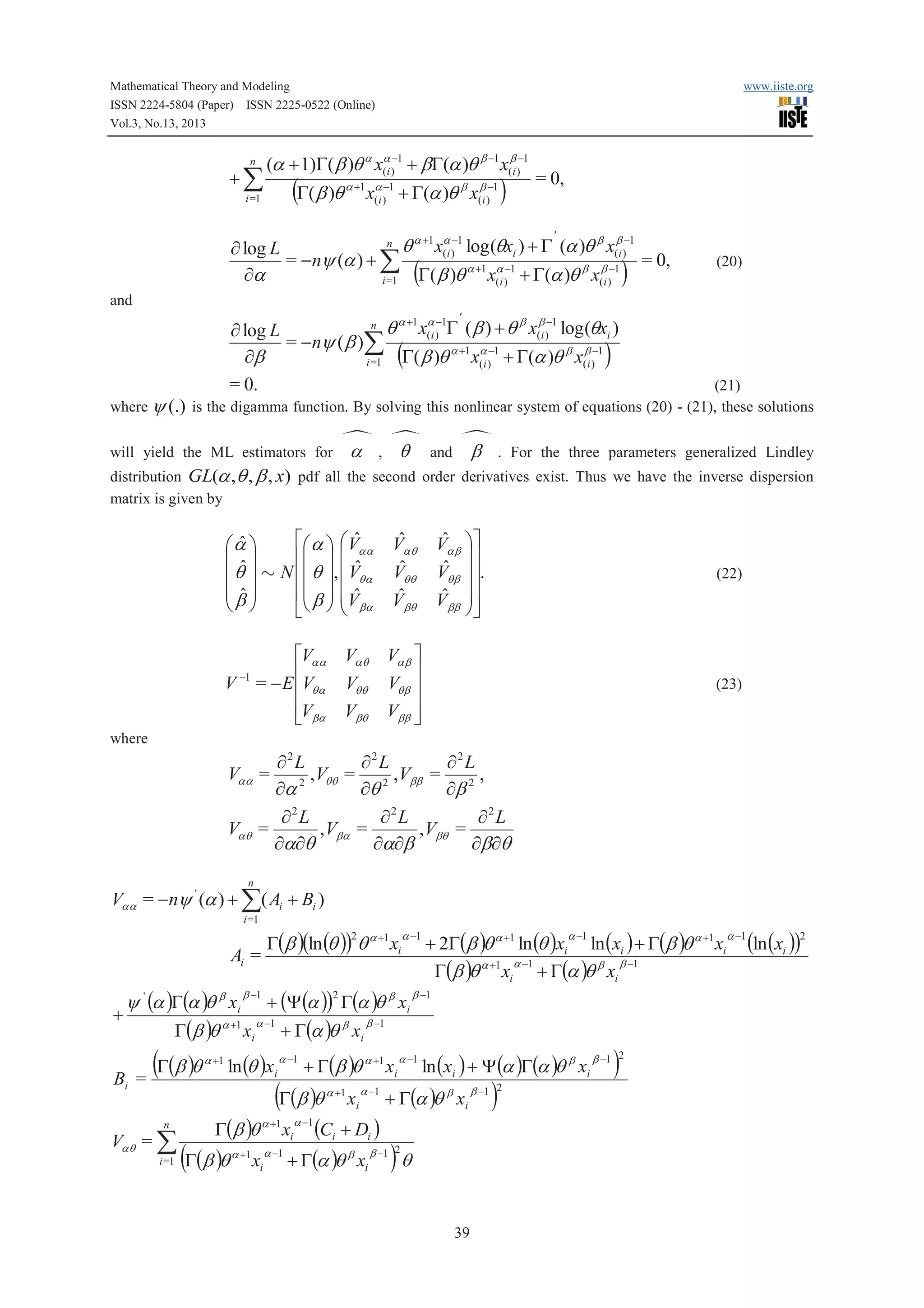
Figure 4: Estimated densities of the models for data set 1.
42](https://image.slidesharecdn.com/anewgeneralizedlindleydistribution-131202193225-phpapp01/75/A-new-generalized-lindley-distribution-13-2048.jpg)
![Mathematical Theory and Modeling
ISSN 2224-5804 (Paper) ISSN 2225-0522 (Online)
Vol.3, No.13, 2013
www.iiste.org
Table 4: The ML estimates, standard error and Log-likelihood for data set 2
Model
Lindley
ML Estimates
St. Error
0.076
ˆ
q = 0.868
ˆ
q = 1.861
NGLD
94.182
0.489
1.238
ˆ
a = 3.585
ˆ = 2.737
b
ˆ
The variance covariance matrix I (l )
computed as
-1
-l
106.928
0.554
of the MLEs under the beta Lindley distribution for data set is
0.569 - 0.001 ö
æ 0.239
÷
ç
1.532 - 0.154 ÷
ç 0.569
ç - 0.001 - 0.154 0.307 ÷
ø
è
ˆ
ˆ
Thus, the variances of the MLE of q , a and b is var(q ) = 0.239,var(a ) = 0.239 and
ˆ
95% confidence
Therefore,
intervals
for
and
are
q ,a
var(b ) = 0.307.
b
[0.901,2.819], [1.158,6.011] and [1.651,3.823] respectively.
Table 5: The AIC, AICC, BIC and K-S of the models based on data set 2
Model
Lindley.
NGLD
- 2l
213.857
188.364
AIC
215.857
194.364
The LR test statistic to test the hypotheses
2
w = 25.493 > 5.991 = c 2;0.05,
AICC
215.942
194.722
BIC
218.133
201.194
K-S
0.232
0.075
/
/
H 0 : a = b = 1 versus H1 : a = 1 Ú b = 1 for data set 2 is
so we reject the null hypothesis. Tables 2 and 4 shows parameter MLEs to
each one of the two fitted distributions for data set 1 and 2, Tables 3 and 5 shows the values of - 2 log( L), AIC,
AICC, BIC and K-S values. The values in Tables 3 and 5, indicate that the new generalized Lindley distribution
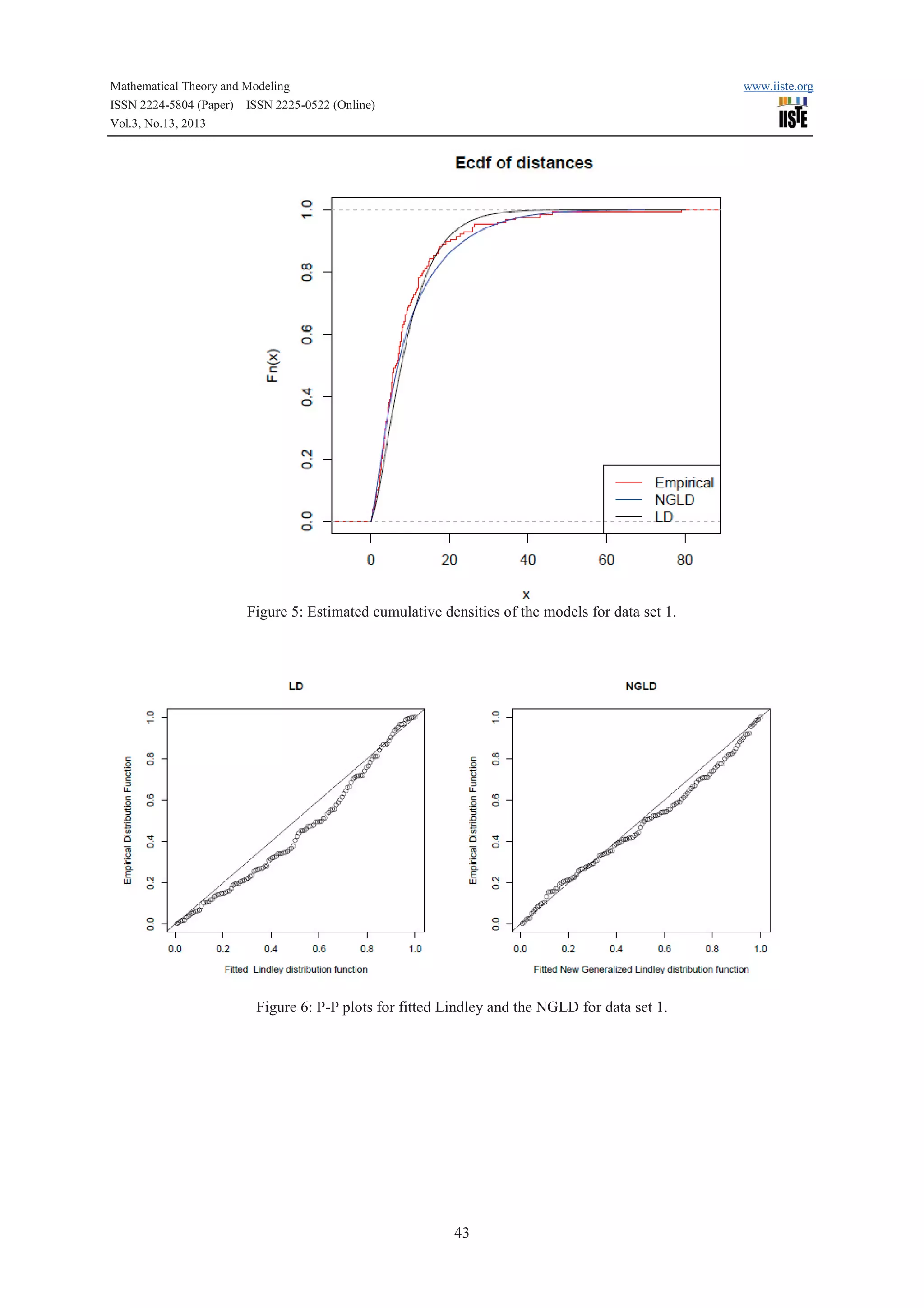
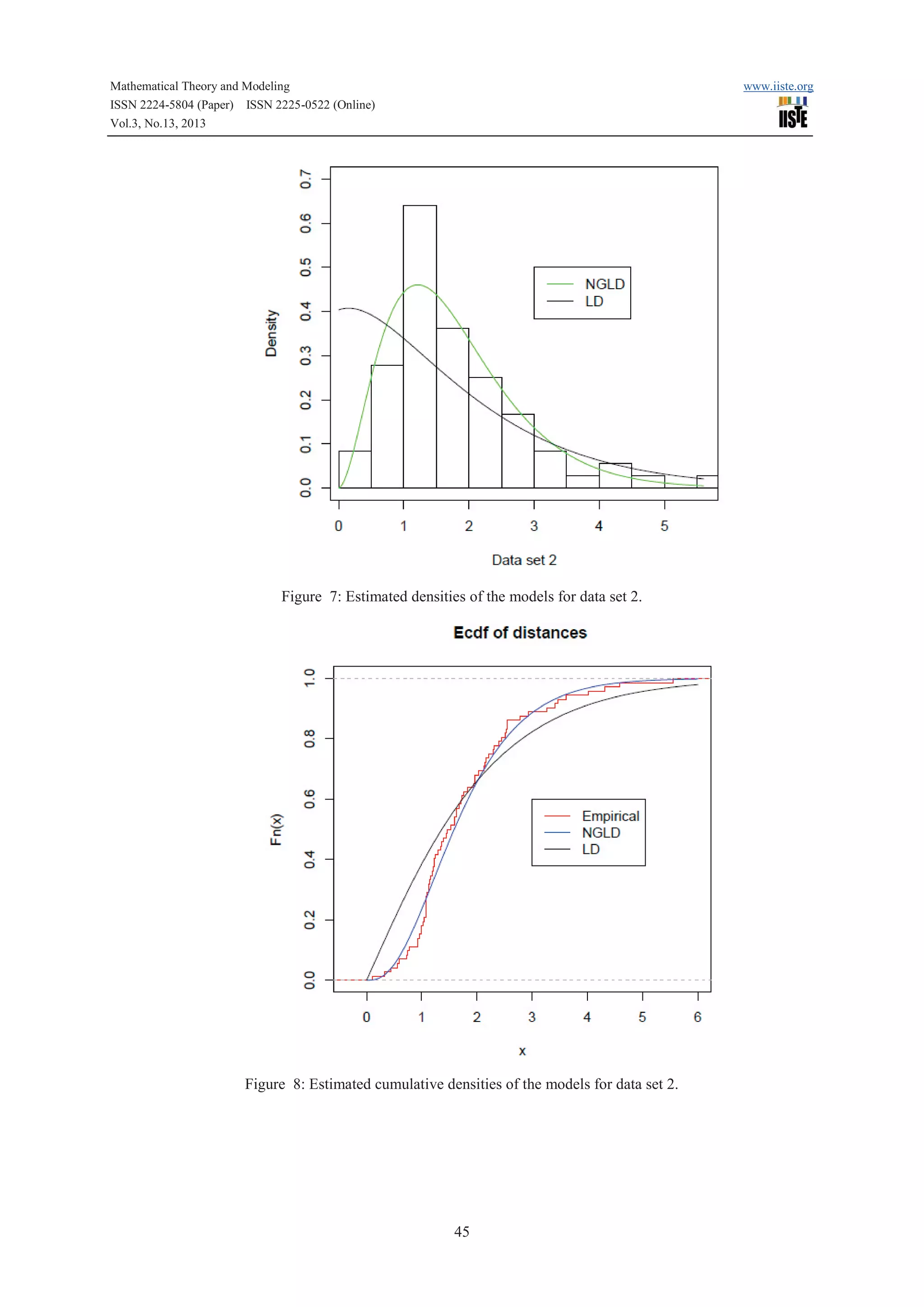
is a strong competitor to other distribution used here for fitting data set 1 and data set 2. A density plot compares
the fitted densities of the models with the empirical histogram of the observed data (Fig. 3 and 5). The fitted
density for the new generalized Lindley model is closer to the empirical histogram than the fits of the Lindley
model.
44](https://image.slidesharecdn.com/anewgeneralizedlindleydistribution-131202193225-phpapp01/75/A-new-generalized-lindley-distribution-15-2048.jpg)
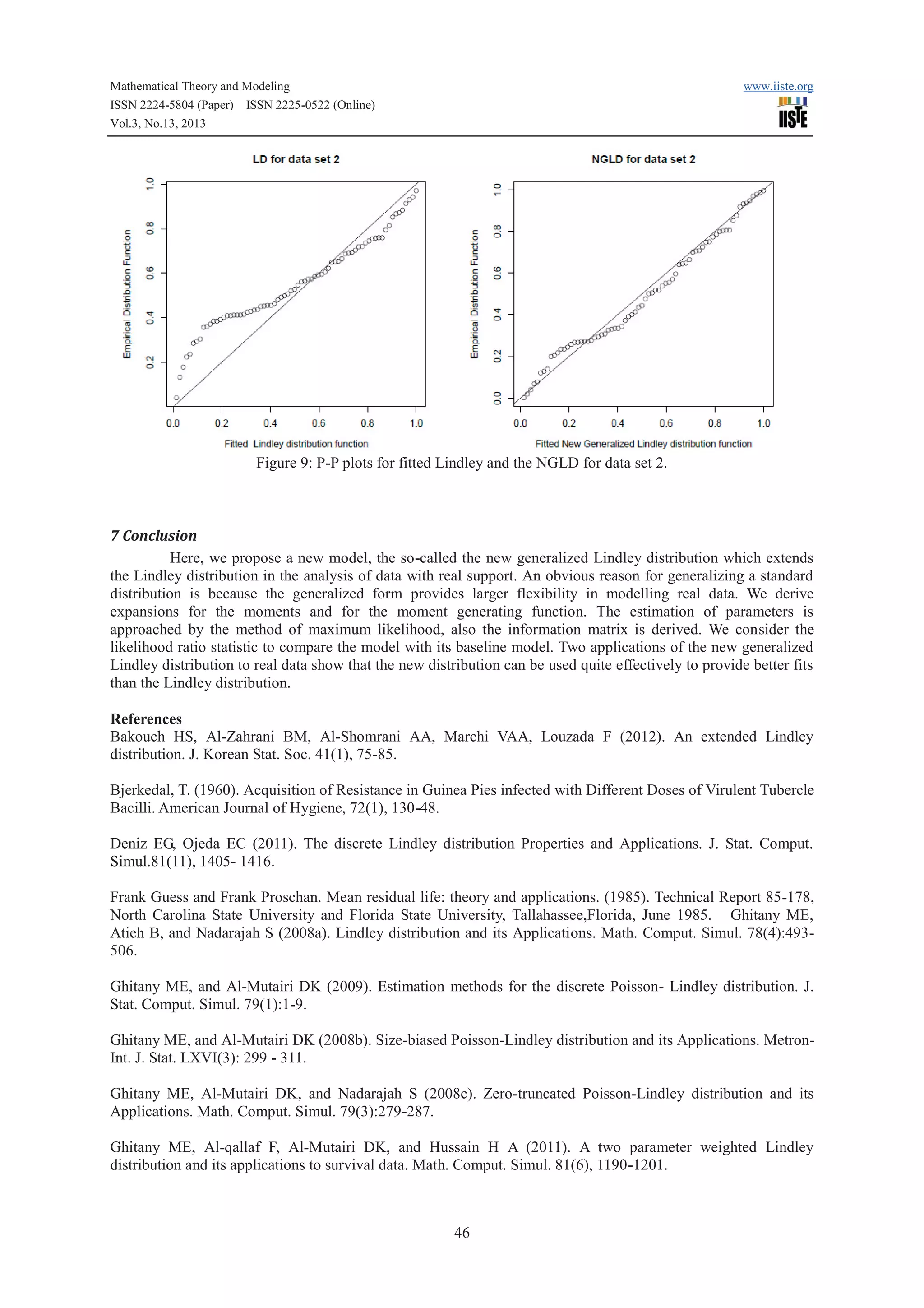


This document presents a new generalized Lindley distribution (NGLD). The NGLD contains the gamma, exponential, and Lindley distributions as special cases. Statistical properties of the NGLD like the hazard function, moments, and moment generating function are derived. Maximum likelihood estimation is discussed to estimate the parameters of the NGLD. Two real data sets are analyzed to illustrate the usefulness of the new distribution.


![Vibe Coding vs. Spec-Driven Development [Free Meetup]](https://cdn.slidesharecdn.com/ss_thumbnails/vibecodingvsspecdrivendevelopment-251209105622-43f455e7-thumbnail.jpg?width=640&height=640&fit=bounds)


