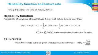
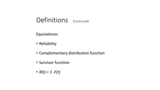
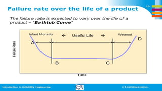
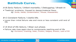
This document discusses key concepts in reliability and safety engineering, including: 1) Defining reliability as a function of time and comparing it to other probability functions like failure distribution and survivor functions. 2) Explaining hazard rates and different failure rate models like Weibull and bathtub curves. 3) Describing the three phases of failure rates over time - infant mortality, steady state, and wear out - and how to model each using distributions.

1. Reliability & Safety Engineering

2. CLO
CO-1: Analyze the fundamental concepts of reliability
CO-2: Interpret the concepts of redundancy and maintenance
CO-3: Compare the various concepts of maintainability
CO-4: Identify the techniques used for of reliability test.
CO-5: Explain the techniques of safety engineering
Unit 1

49. Reliability as a Function of Time
• Reliability R(t): failure occurs after time ‘t’. Let X be
the lifetime of a component subject to failures.
• Let N0: total no. of components (fixed); Ns(t):
surviving ones; Nf(t): failed one by time t.

50. Definitions (Continued)
Equivalence:
• Reliability
• Complementary distribution function
• Survivor function
• R(t) = 1 -F(t)

51. Hazard Rate and the pdf
h(t) t = Conditional Prob. system will fail in
(t, t + t) given that it has survived until time t
f(t) t = Unconditional Prob. System will fail in
(t, t + t)
• Difference between:
• probability that someone will die between 90 and 91, given that he lives to 90
• probability that someone will die between 90 and 91
)
(
1
)
(
)
(
)
(
)
(
t
F
t
f
t
R
t
f
t
h




52. Weibull Distribution
• Frequently used to model fatigue failure, ball bearing failure
etc. (very long tails)
• Reliability:
• Weibull distribution is capable of modeling DFR (α < 1), CFR (α
= 1) and IFR (α >1) behavior.
• α is called the shape parameter and  is the scale parameter
  0

 
t
e
t
R t


53. Failure rate of the weibull
distribution with various values of
 and  = 1
5.0
1.0 2.0 3.0 4.0

54. Infant Mortality Effects in System Modeling
• Bathtub curves
• Early-life period
• Steady-state period
• Wear out period
• Failure rate models

55. Bathtub Curve
Steady State
Infant Mortality
(Early Life Failures) Wear out
•Until now we assumed that failure rate of equipment is time (age)
independent. In real-life, variation as per the bathtub shape has been
observed
Failure
Rate
(t)
Operating Time

56. Early-life Period
• Also called infant mortality phase or reliability
growth phase
• Caused by undetected hardware/software defects
that are being fixed resulting in reliability growth
• Can cause significant prediction errors if steady-
state failure rates are used
• Availability models can be constructed and solved
to include this effect
• Weibull Model can be used

57. Steady-state Period
• Failure rate much lower than in early-life
period
• Either constant (age independent) or slowly
varying failure rate
• Failures caused by environmental shocks
• Arrival process of environmental shocks can
be assumed to be a Poisson process
• Hence time between two shocks has the
exponential distribution

58. • Failure rate increases rapidly with age
• Properly qualified electronic hardware do not
exhibit wear out failure during its intended service
life (Motorola)
• Applicable for mechanical and other systems
• Weibull Failure Model can be used
Wear out Period

59. •We use a truncated Weibull Model
•Infant mortality phase modeled by DFR Weibull and the steady-
state phase by the exponential
0 2,190 4,380 6,570 8,760 10,950 13,140 15,330 17,520
Operating Times (hrs)
Failure-Rate
Multiplier
7
6
5
4
3
2
1
0
Failure Rate Models

60. Failure Rate Models (cont.)
• This model has the form:
• where:
• steady-state failure rate
• is the Weibull shape parameter
• Failure rate multiplier =

 
SS
W t
C
t

 
1
)
(
760
,
8
760
,
8
1



t
t
  
 
 SS
W
C ,
1
1


 SS
W t)
(

61. Failure Rate Models (cont.)
• There are several ways to incorporate time dependent failure rates in
availability models
• The easiest way is to approximate a continuous function by a
decreasing step function
2,190 4,380 6,570 10,950 13,140 15,330 17,520
Operating Times (hrs)
Failure-Rate
Multiplier
7
6
5
4
3
2
1
0
8,760
0
1
2
SS

62. Failure Rate Models (cont.)
•Here the discrete failure-rate model is
defined by:




ss
W t



2
1
)
(
760
,
8
760
,
8
380
,
4
380
,
4
0





t
t
t

63. Uniform Random Variable
• All (pseudo) random generators generate random deviates of U(0,1)
distribution; that is, if you generate a large number of random
variables and plot their empirical distribution function, it will
approach this distribution in the limit.
• U(a,b)  pdf constant over the (a,b) interval and CDF is the ramp
function

64. Uniform density
U(0,1) pdf
0
0.2
0.4
0.6
0.8
1
1.2
0 0.1 0.2 0.3 0.6 0.7 0.8 0.9 1 1.1 1.2 1.3 1.4 1.5 1.6 1.7 1.8 1.9 2 2.1 2.2
time
cdf
0
0.1
0.2
0.3
0.6
0.7
0.8
0.9
1
1.1
1.2
1.3
1.4
1.5
1.6
1.7
1.8
1.9

65. Uniform distribution
• The distribution function is given by:
{
0 , x < a,
F(x)= , a < x < b
1 , x > b.
a
b
a
x



66. Uniform distribution (Continued)
U(0,1) cdf
0
0.2
0.4
0.6
0.8
1
1.2
0
0.08
0.16
0.24
0.32
0.4
0.48
0.56
0.64
0.72
0.8
0.88
0.96
1
1.04
1.08
1.16
1.24
1.32
1.4
1.48
time
cdf
U(0,1) cdf