Download to read offline
![1
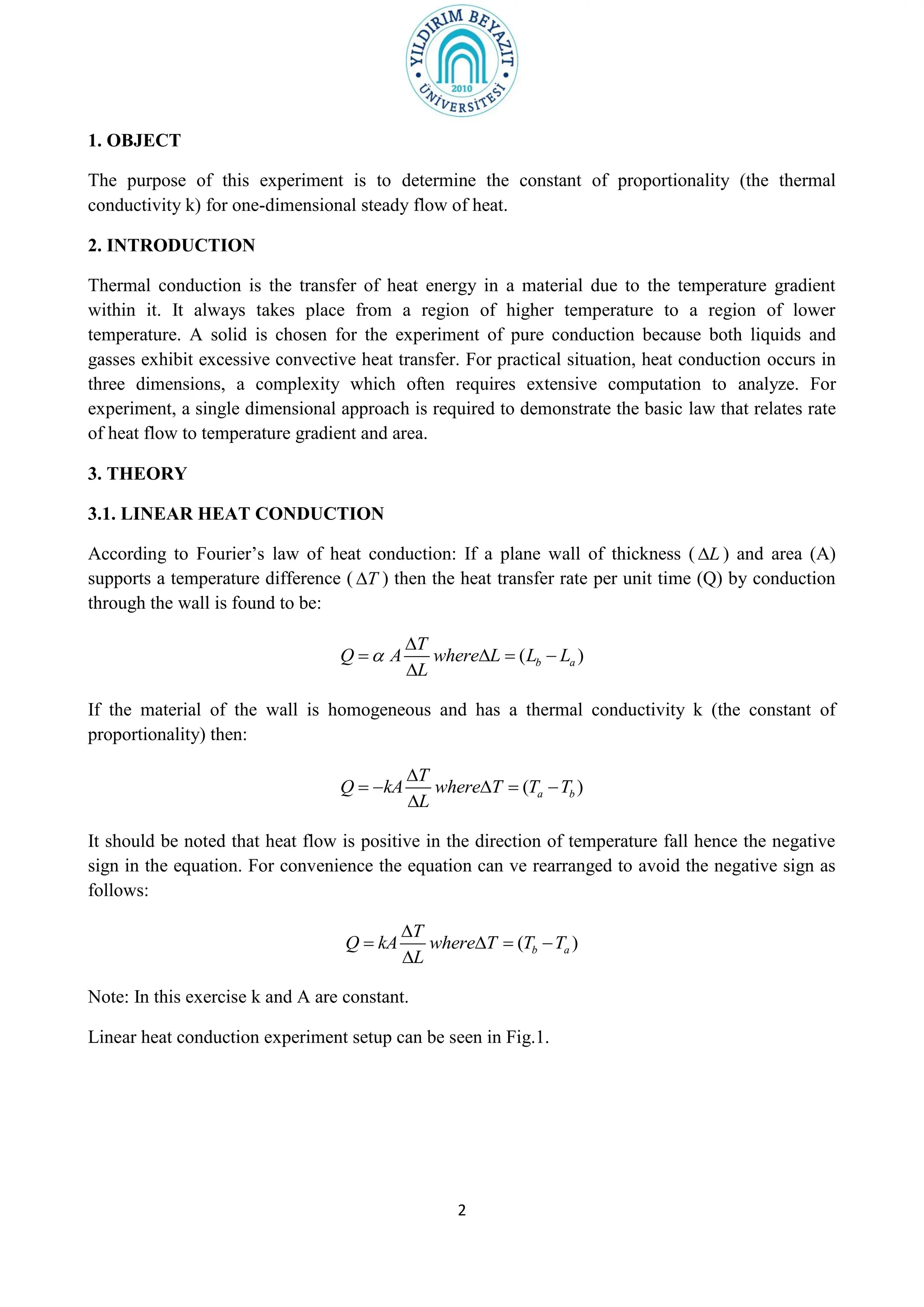
EXPERIMENT: HEAT CONDUCTION
Nomenclature
Name Symbol SI unit
Radius of Disk R [m]
Heat transfer area A [m2
]
Wall thickness (distance) L [m]
Constant Value (k/A) C
Electrical power to heating element Q [W]
Heat transfer rate per unit time (heat flow) Q [W]
Temperature measured Ta (eg. T1) [°C]
Temperature at hot interface Thotface [°C]
Temperature at cold interface Tcoldface [°C]
Temperature gradient Grad (eg. Gradhot) [W/m°C]
Thermal conductivity k [W/m°C]
Time t [secs] α](https://image.slidesharecdn.com/experimentheat-conduction-231202135311-7fc78a9b/75/EXPERIMENT-HEAT-CONDUCTION-pdf-1-2048.jpg)
![6
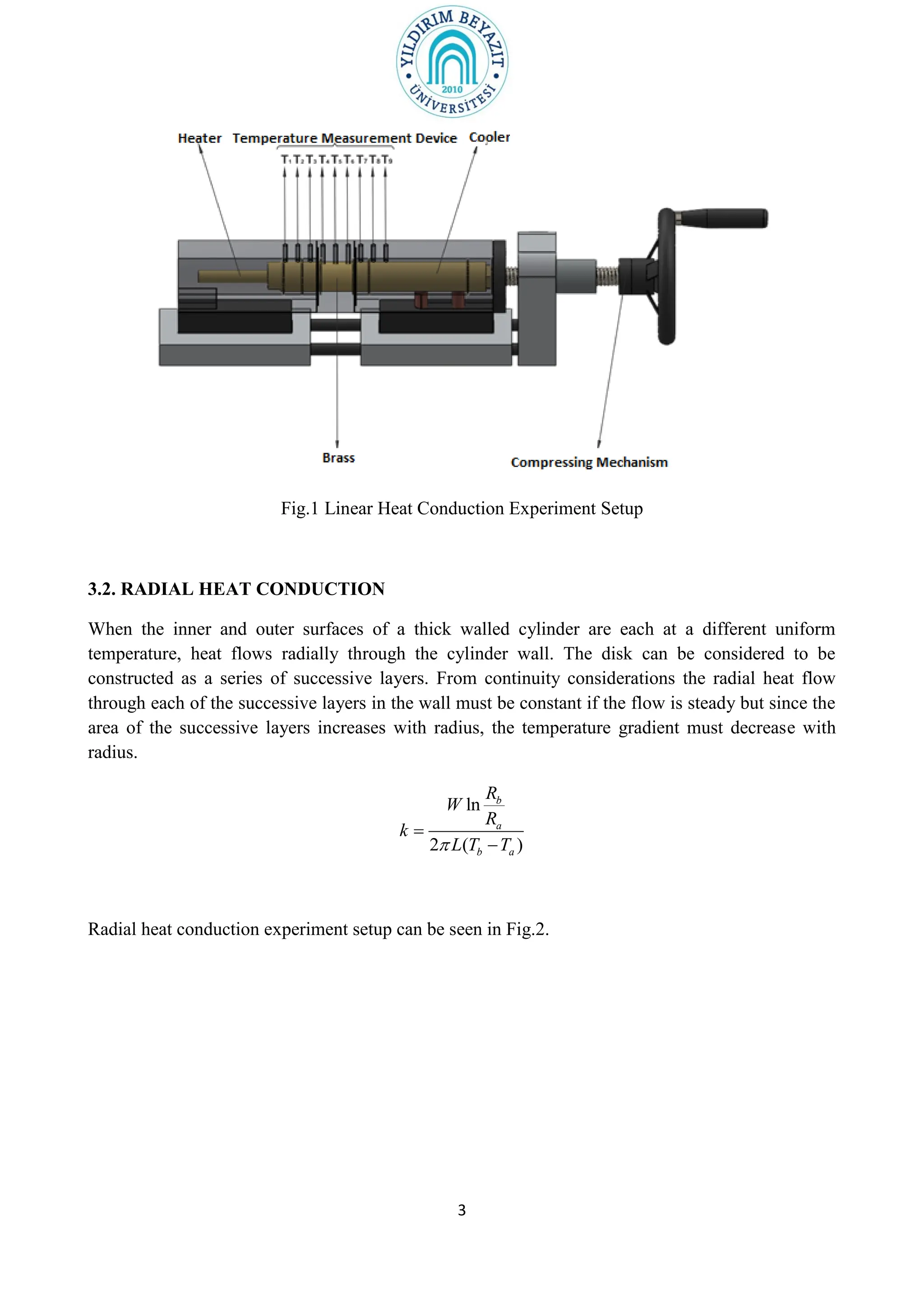
A sample graph of temperature against position along the bar can be seen.
Compare your result with Table 1.
0
10
20
30
40
50
60
70
80
0 1 2 3 4 5 6 7 8
Temperature
[°C]
Distance [m]
Thotface Tcoldface](https://image.slidesharecdn.com/experimentheat-conduction-231202135311-7fc78a9b/75/EXPERIMENT-HEAT-CONDUCTION-pdf-6-2048.jpg)

![9
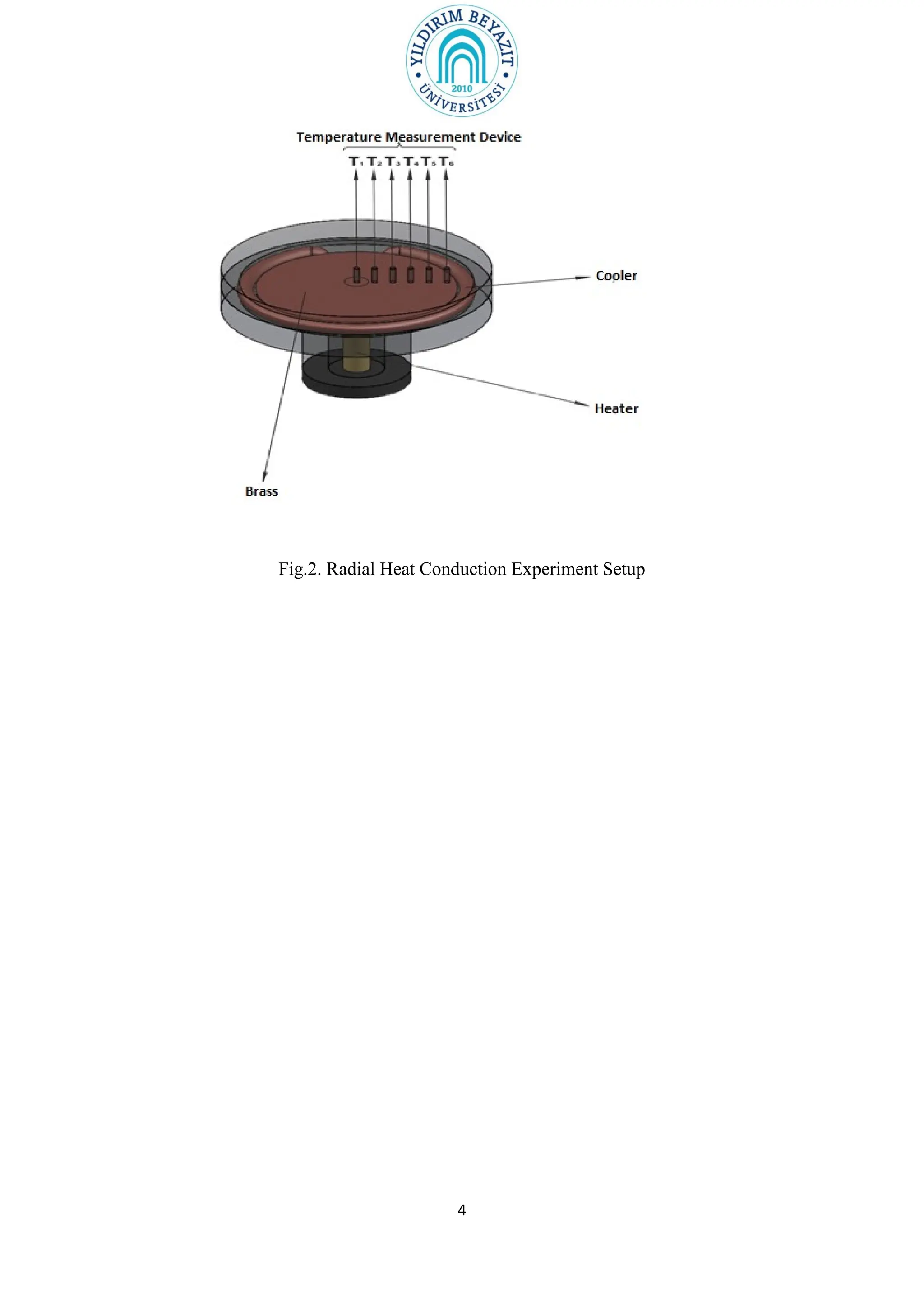
Compare your result with Table 1.
0
10
20
30
40
50
60
70
80
0 1 2 3 4 5 6 7 8
Temperature
[°C]
Distance [m]](https://image.slidesharecdn.com/experimentheat-conduction-231202135311-7fc78a9b/75/EXPERIMENT-HEAT-CONDUCTION-pdf-9-2048.jpg)
![11
0
10
20
30
40
50
60
70
80
0 1 2 3 4 5 6 7 8
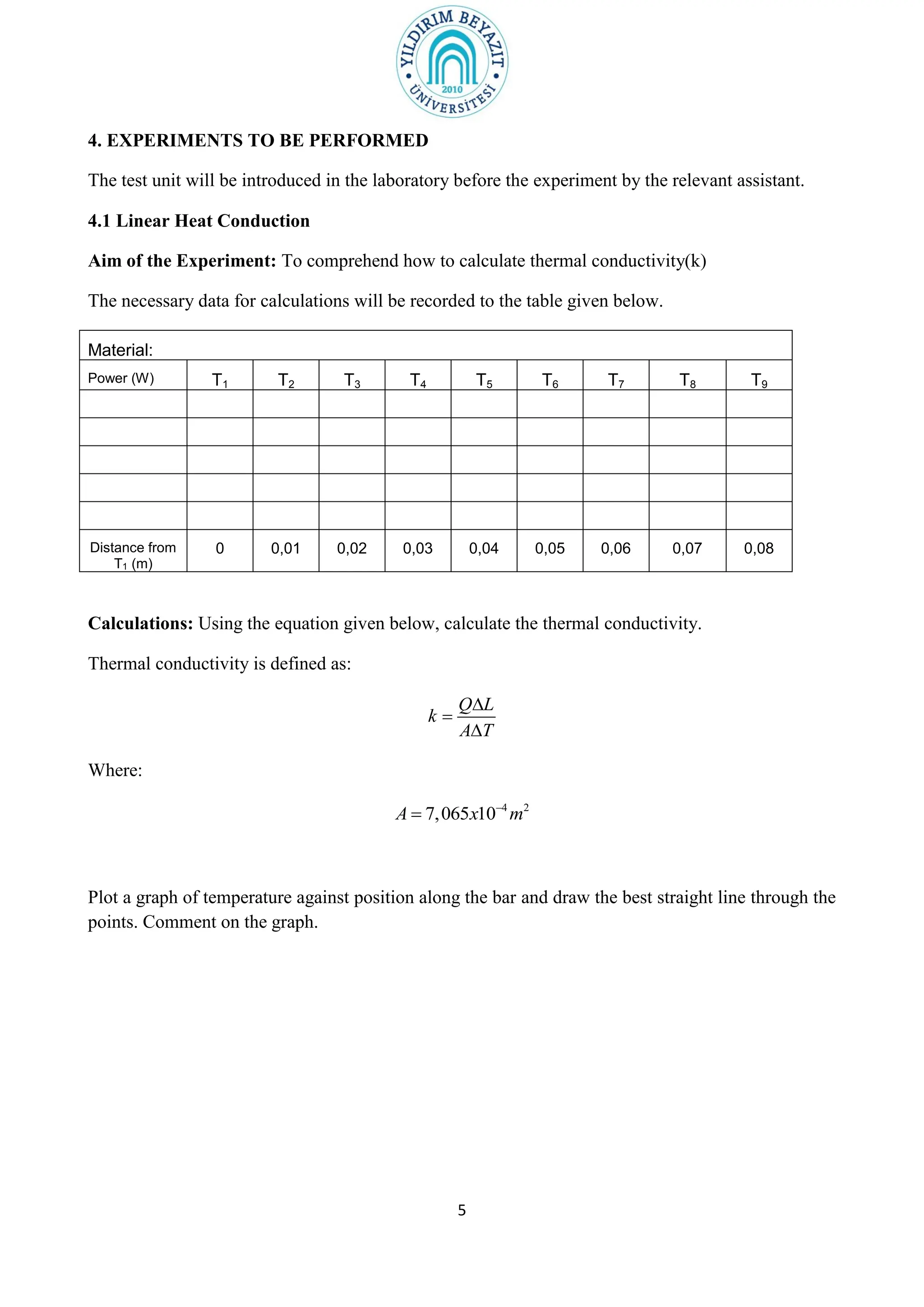
Temperature
[°C]
Radial Distance [m]](https://image.slidesharecdn.com/experimentheat-conduction-231202135311-7fc78a9b/75/EXPERIMENT-HEAT-CONDUCTION-pdf-11-2048.jpg)


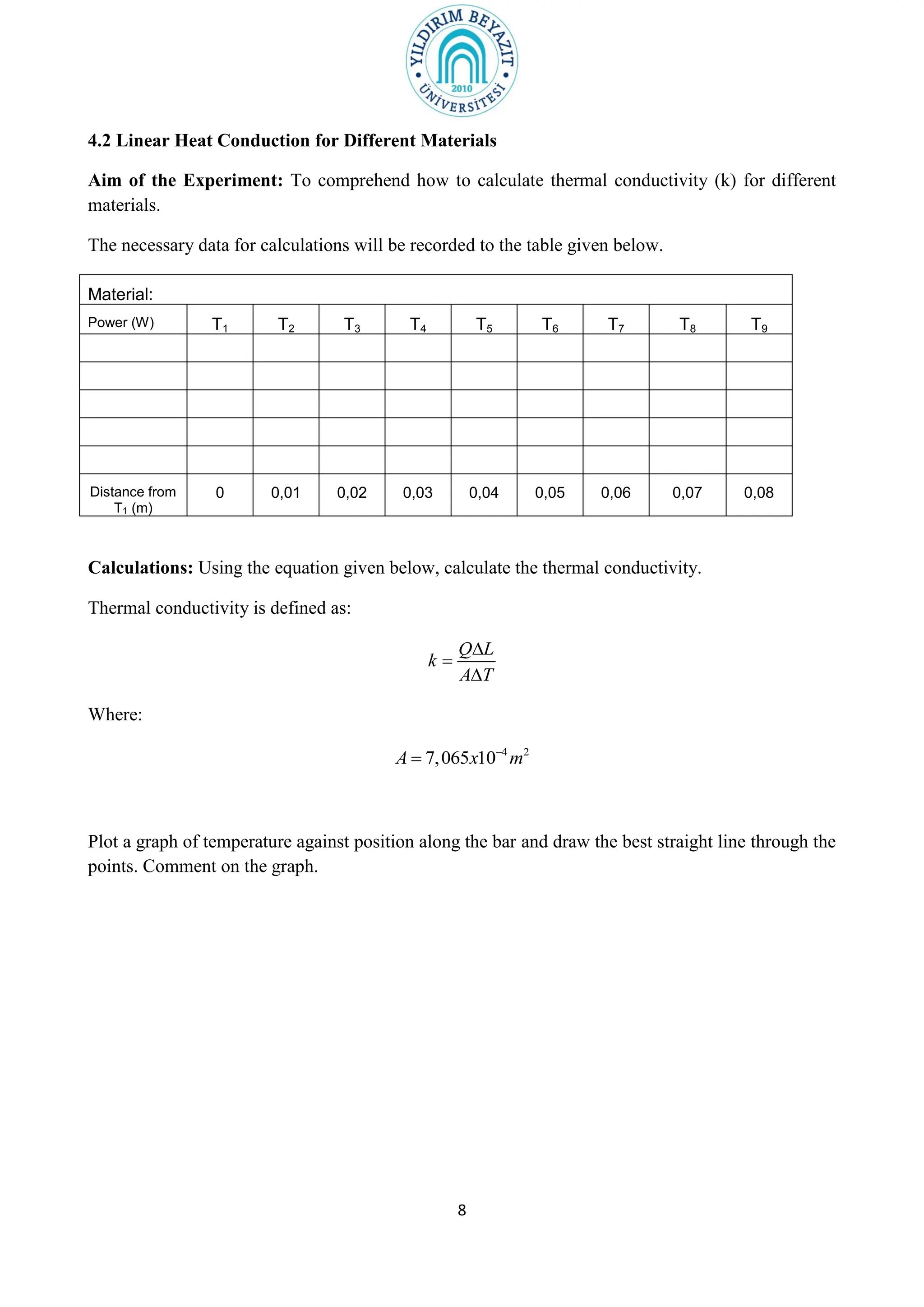
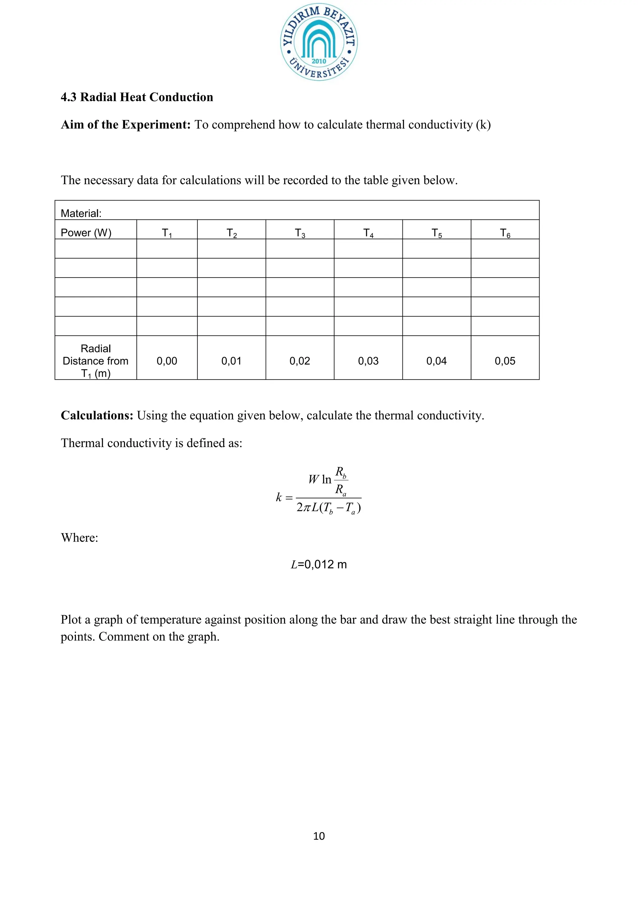
1. The purpose of the experiment is to determine the thermal conductivity (k) of materials using linear and radial heat conduction. 2. The document outlines the theory of linear and radial heat conduction according to Fourier's law. It provides the equations to calculate thermal conductivity based on heat transfer rate, temperature gradient, thickness/radius, and area. 3. The experiment procedures involve measuring temperature gradients across materials and calculating k for different materials using the provided equations. Graphs of temperature vs. position will also be analyzed to determine k. Results will be reported and compared to literature values.


