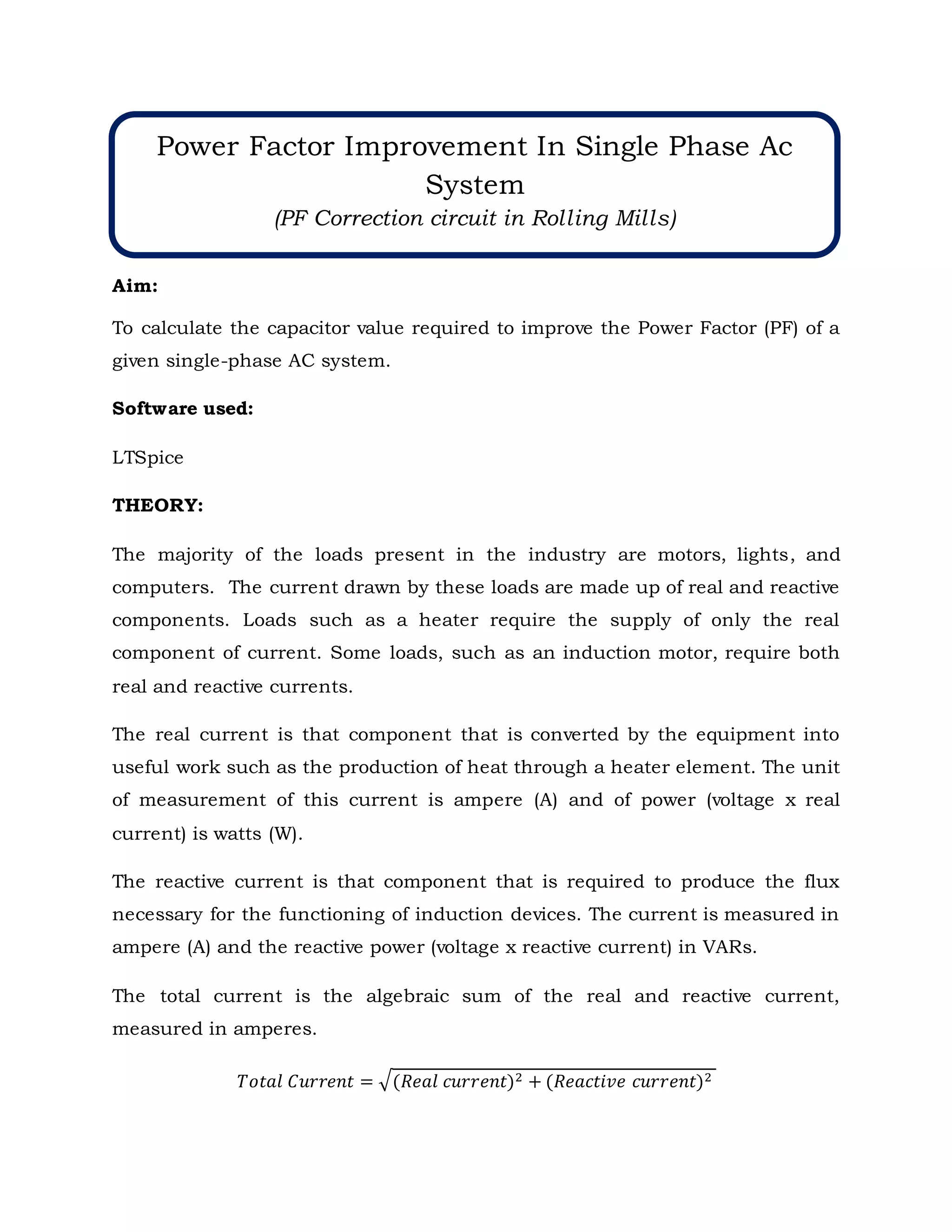
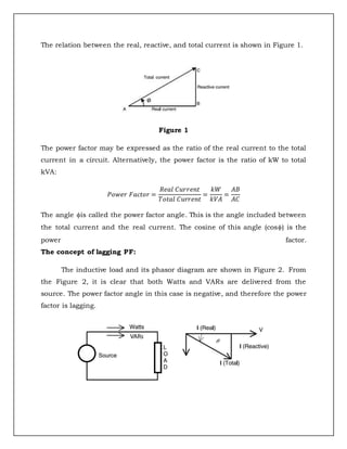
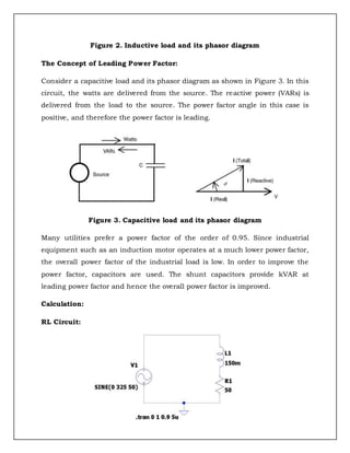
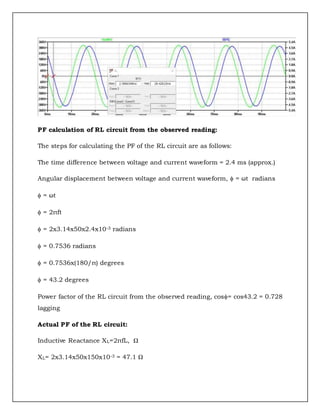
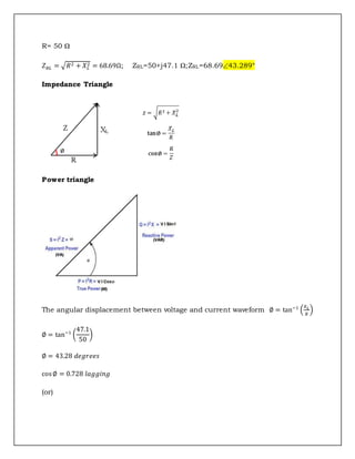
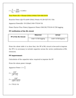
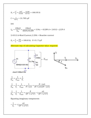
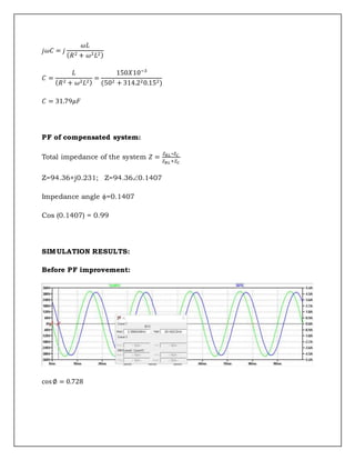
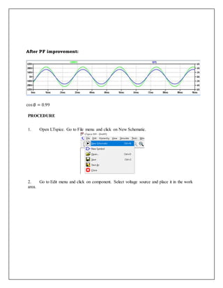
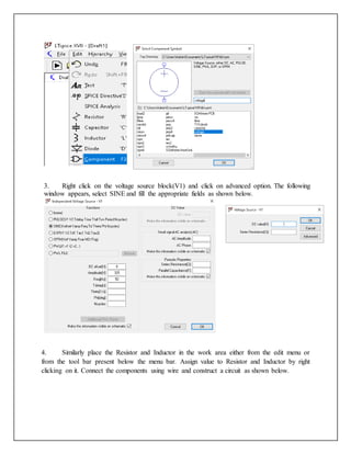
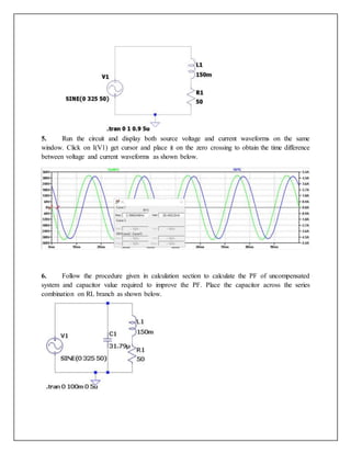
To calculate the capacitor value required to improve the power factor of a single-phase AC system. The document discusses power factor in inductive and capacitive loads, defines true power, reactive power and apparent power. It then shows calculations for an RL circuit's power factor and determining the required capacitor value to improve the power factor. Simulations in LTSpice are used to verify the calculated capacitor value improves the power factor from 0.728 to 0.99 lagging.

1. Aim:
To calculate the capacitor value required to improve the Power Factor (PF) of a
given single-phase AC system.
Software used:
LTSpice
THEORY:
The majority of the loads present in the industry are motors, lights, and
computers. The current drawn by these loads are made up of real and reactive
components. Loads such as a heater require the supply of only the real
component of current. Some loads, such as an induction motor, require both
real and reactive currents.
The real current is that component that is converted by the equipment into
useful work such as the production of heat through a heater element. The unit
of measurement of this current is ampere (A) and of power (voltage x real
current) is watts (W).
The reactive current is that component that is required to produce the flux
necessary for the functioning of induction devices. The current is measured in
ampere (A) and the reactive power (voltage x reactive current) in VARs.
The total current is the algebraic sum of the real and reactive current,
measured in amperes.
𝑇𝑜𝑡𝑎𝑙 𝐶𝑢𝑟𝑟𝑒𝑛𝑡 = √(𝑅𝑒𝑎𝑙 𝑐𝑢𝑟𝑟𝑒𝑛𝑡)2 + (𝑅𝑒𝑎𝑐𝑡𝑖𝑣𝑒 𝑐𝑢𝑟𝑟𝑒𝑛𝑡)2
Power Factor Improvement In Single Phase Ac
System
(PF Correction circuit in Rolling Mills)

2. The relation between the real, reactive, and total current is shown in Figure 1.
Figure 1
The power factor may be expressed as the ratio of the real current to the total
current in a circuit. Alternatively, the power factor is the ratio of kW to total
kVA:
𝑃𝑜𝑤𝑒𝑟 𝐹𝑎𝑐𝑡𝑜𝑟 =
𝑅𝑒𝑎𝑙 𝐶𝑢𝑟𝑟𝑒𝑛𝑡
𝑇𝑜𝑡𝑎𝑙 𝐶𝑢𝑟𝑟𝑒𝑛𝑡
=
𝑘𝑊
𝑘𝑉𝐴
=
𝐴𝐵
𝐴𝐶
The angle is called the power factor angle. This is the angle included between
the total current and the real current. The cosine of this angle (cos) is the
power factor.
The concept of lagging PF:
The inductive load and its phasor diagram are shown in Figure 2. From
the Figure 2, it is clear that both Watts and VARs are delivered from the
source. The power factor angle in this case is negative, and therefore the power
factor is lagging.

3. Figure 2. Inductive load and its phasor diagram
The Concept of Leading Power Factor:
Consider a capacitive load and its phasor diagram as shown in Figure 3. In this
circuit, the watts are delivered from the source. The reactive power (VARs) is
delivered from the load to the source. The power factor angle in this case is
positive, and therefore the power factor is leading.
Figure 3. Capacitive load and its phasor diagram
Many utilities prefer a power factor of the order of 0.95. Since industrial
equipment such as an induction motor operates at a much lower power factor,
the overall power factor of the industrial load is low. In order to improve the
power factor, capacitors are used. The shunt capacitors provide kVAR at
leading power factor and hence the overall power factor is improved.
Calculation:
RL Circuit:

4. PF calculation of RL circuit from the observed reading:
The steps for calculating the PF of the RL circuit are as follows:
The time difference between voltage and current waveform = 2.4 ms (approx.)
Angular displacement between voltage and current waveform,  = ωt radians
 = ωt
 = 2πft
 = 2x3.14x50x2.4x10-3 radians
 = 0.7536 radians
 = 0.7536x(180/π) degrees
 = 43.2 degrees
Power factor of the RL circuit from the observed reading, cos= cos43.2 = 0.728
lagging
Actual PF of the RL circuit:
Inductive Reactance XL=2πfL, Ω
XL= 2x3.14x50x150x10-3 = 47.1 Ω

5. R= 50 Ω
𝑍𝑅𝐿 = √𝑅2 + 𝑋𝐿
2 = 68.69Ω; ZRL=50+j47.1 Ω;ZRL=68.6943.289°
Impedance Triangle
Power triangle
The angular displacement between voltage and current waveform ∅ = tan−1
(
𝑋𝐿
𝑅
)
∅ = tan−1
(
47.1
50
)
∅ = 43.28 𝑑𝑒𝑔𝑟𝑒𝑒𝑠
cos∅ = 0.728 𝑙𝑎𝑔𝑔𝑖𝑛𝑔
(or)

6. 𝐼 =
𝑉
𝑍𝑅𝐿
=
230
68.69
= 3.348 𝐴
True Power (P) = VIcos=230x3.348x0.728=560.58 W
Reactive Power (Q)=VI sinΦ=230x3.34xsin 43.28=527.911 VAr
Apparent Power(S)= VI=230x3.348=770.04 VA
Power Factor=True Power/Apparent Power=560.58/770.04=0.728 lagging
PF verification of the RL circuit
PF of the RL Circuit
Observed Actual
cos= 0.728 lagging cos∅ = 0.728 𝑙𝑎𝑔𝑔𝑖𝑛𝑔
From the above table it is clear that, the PF of RL circuit is low and to improve
the PF it is necessary to include capacitor across the series combination of RL
elements.
PF improvement:
Calculation of the capacitor value required to improve the PF
From the above power triangle
Apparent Power 𝑆 =
𝑉2
𝑍
𝑆 =
2302
√𝑅2 + 𝑋𝐿
2
𝑆 =
2302
√502 + 47.12
𝑆 = 770.12 𝑉𝐴

7. 𝑋𝐶 =
𝑉2
𝑄
=
2302
𝑉𝐼𝑠𝑖𝑛∅
=
52,900
527 .911
= 100.195 Ω
𝐶 =
1
2𝜋𝑓𝑋𝑐
= 31.785 μF
(or)
𝐼𝑅𝐿 =
230∠0
𝑍𝑅𝐿
=
230∠0
68.69∠43.289
= 3.34∠ − 43.289 𝐴 = 2.4312 − 𝑗2.29 𝐴
2.4312 A=Real Current; 2.29A = Reactive current
𝑋𝐶 =
𝑉
𝐼𝐶
=
230
2.29
= 100.43 Ω; C=31.71μF
Alternate way of calculating Capacitor value required:
1
𝑍𝑒𝑞
=
1
𝑍𝑙𝑜𝑎𝑑
+
1
𝑍𝑐
1
𝑍𝑒𝑞
−
1
𝑍𝑐
=
1
𝑍𝑙𝑜𝑎𝑑
=
1
𝑅 + 𝑗𝜔𝐿
=
𝑅 − 𝑗𝜔𝐿
(𝑅 + 𝑗𝜔𝐿)(𝑅 − 𝑗𝜔𝐿)
1
𝑍𝑒𝑞
−
1
𝑍𝑐
=
1
𝑍𝑙𝑜𝑎𝑑
=
𝑅
(𝑅2 + 𝜔2 𝐿2)
− 𝑗
𝜔𝐿
(𝑅2 + 𝜔2𝐿2)
Equating imaginary components
−
1
𝑍𝑐
= −𝑗
𝜔𝐿
(𝑅2 + 𝜔2𝐿2)

8. 𝑗𝜔𝐶 = 𝑗
𝜔𝐿
(𝑅2 + 𝜔2𝐿2)
𝐶 =
𝐿
(𝑅2 + 𝜔2𝐿2)
=
150𝑋10−3
(502 + 314.220.152)
𝐶 = 31.79𝜇𝐹
PF of compensated system:
Total impedance of the system 𝑍 =
𝑍𝑅𝐿 ∗𝑍𝐶
𝑍𝑅𝐿 +𝑍𝐶
Z=94.36+j0.231; Z=94.360.1407
Impedance angle =0.1407
Cos (0.1407) = 0.99
SIMULATION RESULTS:
Before PF improvement:
cos∅ = 0.728

9. After PF improvement:
cos∅ = 0.99
PROCEDURE
1. Open LTspice. Go to File menu and click on New Schematic.
2. Go to Edit menu and click on component. Select voltage source and place it in the work
area.

10. 3. Right click on the voltage source block(V1) and click on advanced option. The following
window appears, select SINE and fill the appropriate fields as shown below.
4. Similarly place the Resistor and Inductor in the work area either from the edit menu or
from the tool bar present below the menu bar. Assign value to Resistor and Inductor by right
clicking on it. Connect the components using wire and construct a circuit as shown below.

11. 5. Run the circuit and display both source voltage and current waveforms on the same
window. Click on I(V1) get cursor and place it on the zero crossing to obtain the time difference
between voltage and current waveforms as shown below.
6. Follow the procedure given in calculation section to calculate the PF of uncompensated
system and capacitor value required to improve the PF. Place the capacitor across the series
combination on RL branch as shown below.

12. 7. Run the circuit and verify the improvement in the PF value by following the steps given
in calculation section.
Result:
Results and Inferences:
Practical Applications:
Used for PF correction in Industry
Course Outcome:
CO2. Analyze AC power circuits and networks, its measurement and safety concerns
Student Learning Outcomes (SLO):
SLO2. Having a clear understanding of the subject related concepts and of contemporary
issues
SLO9. Having problem solving ability- solving social issues and engineering problems