This document discusses evaporation effects on inkjet performance and image quality. It summarizes that as nozzles sit idle, water evaporation causes large localized viscosity variations in the inkjet ejector. This has a negative impact on jetting performance and print quality. The document then goes into detail explaining the multi-physics involved, including heat and mass convection/diffusion at the ink-air interface, and how this affects the transient viscosity fields and ultimately jetting and image quality. Models are used to predict and understand these relationships and tradeoffs between ink formulation, environmental effects, and ejector design.

1. Print Physics Notes: Evaporation Effects on Inkjet Performance and Image Quality
December 2008
1
Evaporation Effects on Inkjet Performance and Print Quality
Robert W. Cornell; Print Systems Science; Lexmark International; Lexington, Kentucky
Abstract
As nozzles sit idle, water evaporation causes large, highly
localized viscosity variations in an inkjet ejector. This has long
been a topic of qualitative discussion and empirical studies. This
analysis goes to the root of the problem, covering the underlying
multi-physics at work, the mathematical solution techniques and
model validations at each step along the way.
It is shown that significant viscosity field variations occur in
the ejector on a time scale less than one second. Idle time
evaporation induced viscosity variations have a negative impact on
jetting performance and print quality. This article examines this
phenomenon quantitatively. It begins with a discussion on the
properties of moist air and continues on to the topics; heat and
mass convection/diffusion. The boundary layer equations for heat
and mass transfer in the gap between a swathing print-head and a
media surface are derived, as are the resultant convection
coefficients. It is shown that the mass convection coefficient is
inversely proportional to media gap – a result that helps explain
machine-machine idle time variation. Also, a method is presented
to predict viscosity and mass diffusivity properties for multi-
component ink- mixtures as a function of formulation, temperature
and water loss. Next an overview of the finite element method is
presented to illustrate the solution means for the field equations.
Evaporative flux exiting an inkjet ejector is then discussed from
experimental and theoretical viewpoints. It will be shown that a
heretofore undiscovered mechanism is at work during the first few
seconds of evaporation. This mechanism tends to cause the
evaporation rate from an inkjet nozzle to be self-limiting. The
experimental and simulation results agree quite well on this
phenomenon. The evaporation and mass diffusion results are then
merged with the jetting model. The temporal and spatial variations
of viscosity are accounted for, enabling the jetting model to predict
the idle time print quality defects – drop placement error and
reflective luminance variation. The predicted idle time defects are
very much on target with experimental results. Lastly, the pigment-
dye dilemma is quantitatively discussed as are the paths that some
competitors have taken to enable idle time robustness with pigment
inks.
Introduction
An uncapped, idle nozzle will suffer water loss by evaporation.
After a few seconds, or less, the remnant mixture in the nozzle
consists primarily of highly viscous co-solvents. While all inks are
affected by evaporation, the negative impact on performance is
magnified with pigment inks. HP has expressed similar thoughts
on this. “Pigment inks cannot be de-capped for more than a few
seconds without significant property changes, so Edgeline spits all
nozzles after ~800ms of idle time.” [1]
Within seconds, the physical properties of the ink change well
beyond the range needed for consistent jetting. The resulting weak
and misdirected droplets are easily visible and highly objectionable
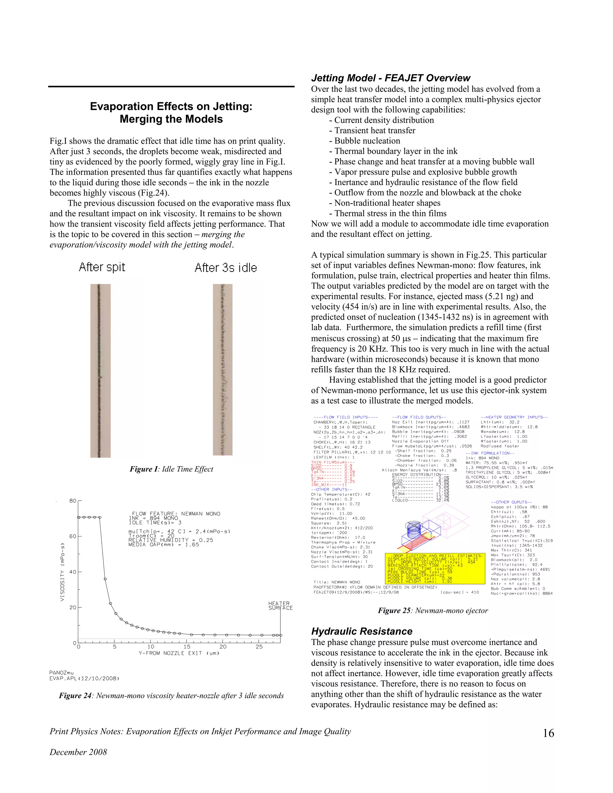
from a print quality viewpoint. Fig.I illustrates this effect.
Figure I: Idle Time Effect
This article examines and quantifies the interrelationships
between the ejector flow features, local environmental conditions,
media gap and ink formulation choices that impact the transient
mass diffusion and viscosity fields, and ultimately – how these
affect jetting and imaging performance.
The goal of all mathematical models is to predict performance
of some variable set [ as a function of a wide variety of inputs.
In some simple cases, the model results lead to optimum,
bulletproof designs. However, like most things inkjet, there is no
“optimum” design for idle time. Rather, there exists a series of
tradeoffs where one parameter suffers at the expense of another.
That is not to say modeling is an esoteric exercise. Indeed, exactly
the opposite is the case. When a simple system is designed for
optimum performance it is often easy to do so with minimal
experimentation and computation. However, when the system
involves a complex set of field variables covering many scientific
disciplines, it may take decades of experimentation to build a
disconnected set of empirical do/don’t rules. When the modeling
approach is not easily accomplished because of complex
mathematical physics, the variables also are usually so endless that
full-factorial experiments are utterly impractical. In such cases,
taking the time to develop a mathematical model is extremely
important, and well-worth the effort, because it permits tradeoffs to
be studied without decades of empiricism. That said, the value of
the multi-physics model described herein is a means of quantifying
idle time tradeoffs between: ink formulation, environmental
effects, thermo-hydrodynamic ejector effects, jetting and image
quality.
Properties of Moist Air
Evaporation may be rate-limited by any of the following [2]:
 Vapor diffusion across a stagnant, or non-receptive gas
layer above the liquid

2. Print Physics Notes: Evaporation Effects on Inkjet Performance and Image Quality
December 2008
2
 A barrier that impedes molecular transport at the liquid-
vapor surface
 Evaporation of a volatile species may generate
concentration gradients in the liquid such that mass
transport within the liquid is rate-limiting
Since vapor diffusion is dependent upon the gas properties existing
in the boundary layer at the liquid-air interface, a good starting
point for this analysis is psychrometrics [3].
Moist air is a binary mixture of dry air and water vapor.
Humidity ratio (W) is the mass of water vapor per unit mass of dry
air. Since it is known that dry air has a molecular weight of 29
grams/mol and water vapor has a molecular weight of 18
grams/mol, it is convenient to write the following expression for
humidity ratio.



















W
W
W
W
x
x
x
x
W
1
622.0
129
18
(Eq.1)
xW = mol-fraction water vapor contained in the moist air
Relative humidity () is also conveniently related to water vapor
mol fraction:
SW
W
x
x
,
 (Eq.2)
xW = mol-fraction water vapor contained within the air at Troom
Troom = room temperature
xW,S = mol-fraction water vapor at saturation at Troom
Using Dalton’s Rule, (Eqs.1-2) can be written in terms of pressure.
pressurecatmospheri
airmoistinorwater vapofpressurepartial
622.0






P
P
PP
P
W
W
W
W
(Eq.3)
Standard atmospheric pressure = 101300 (N/m2
) = 101300 (Pa)
SW
W
P
P
,
 (Eq.4)
PW,S = saturated vapor pressure(TROOM , 100% relative humidity)
Then the saturated humidity ratio (WS) can be written:
SW
SW
S
PP
P
W
,
,
622.0



(Eq.5)
Pressure values may be obtained from look-up steam tables, or
they may be computed from the ideal gas law approximation of the
Clausius-Clapeyron equation, shown below.












 
TTbR
hfgM
PTP
11
exp)( (Eq.6)
P(T) = vapor pressure (Pascal, or N/m2
) at temperature (T)
hfg = latent heat of evaporation = 2.35 x 106
(J/Kg) for water
M = molecular weight = 0.018 (Kg/mol) for water
R = universal gas constant = 8.315 (J/mol-K)
Tb = normal boiling temperature = 373 (K) for water
T = temperature (K)
Consequently, saturated temperature values may be computed by
rearranging (Eq.6):
   
      


















P
P
RTbMhfg
MhfgTb
PT
ln
)( (Eq.7)
T(P) = saturated vapor temperature (K) at vapor pressure [P(Pa)]
Eq.6 compares favorably to steam table values, as shown in Fig.1.
Figure 1: Vapor pressure versus water temperature
Example
If the room temperature is 25C, and the relative humidity is 35%;
find the saturated vapor pressure (PW,S), the partial pressure of
water vapor in the moist air (PW), the humidity ratio (W), the
saturated humidity ratio (WS) and the dew point temperature
(TDEW).
By (Eq.6) the saturated vapor pressure at 25C is:
PW,S(298K) = 3272 Pa = 24 mm-Hg
By (Eq.4) the partial pressure of water vapor at 25C and 35%
relative humidity is:
PW(298K, 0.35) = 1145 Pa = 8.6 mm-Hg
By (Eq.3) the humidity ratio of air at 25C and 35% relative
humidity is:
W = 0.007 Kg-water/Kg-dry air
By (Eq.5) the saturated humidity ratio at 25C is:
Ws = 0.0208 Kg-water/Kg-dry air
By (Eq.7) the dew point temperature at a dry bulb temperature of
25C and 35% relative humidity is:
TDEW = 281K = 8C
These values may also be extracted from a psychrometric chart
(Fig. 2-3), but for mathematical convenience it is more desirable to
use (Eq.1-7).

3. Print Physics Notes: Evaporation Effects on Inkjet Performance and Image Quality
December 2008
3
Figure 2: Psychrometric Chart
Figure 3: Psychrometric Chart-Expanded
Heat and Mass Convection
Now let us discuss the kinetics of water evaporation into moist air.
During typical evaporation, heat is transferred from the air into the
water, and mass (water vapor) is transferred from the liquid into
the air. The energy transfer process occurring at the liquid-air
interface is heat-convection and heat-conduction, while the
evaporative transfer process is mass-convection and mass-
diffusion.
Heat transfer at the vapor-liquid interface obeys the following
relationship:
 
Surfacey
SROOMC
y
T
kTThq









 (Eq.8)
q = heat flux (W/m2
)
hC = heat transfer convection coefficient (W/m2
-C)
TROOM = room temperature (C)
TS = temperature at the liquid surface (C)
k = thermal conduction coefficient of air (W/m-C)
Similarly, mass transfer at the vapor-liquid interface is described
by:
 
fluxmassareaunitperunit timepertransfermass
:Where
0





























A
m
y
W
DWWh
A
m
y
AIRAIRSD 
(Eq.9)
hD = mass convection coefficient (Kg/m2
-s)
DAIR = water vapor-air diffusion coefficient (m2
/s)
AIR = density of air (Kg/m3
)
y = 0 is the vapor-liquid interface
Note: it is obvious from (Eq.3) and (Eq.5) that (Eq.9) can
also be written in terms of vapor pressure and pressure
gradient, as often seen in the literature.
It can be shown that the mass diffusion coefficient (hD) is related to
the heat transfer convection coefficient (hC) by [4]:
  3
2
3/2
Le
DCph
h
AIR
AIR
AIRD
C










(Eq.10)
CpAIR = specific heat of air (J/Kg-C)
AIR = thermal diffusivity of air (m2
/s)
The ratio of thermal diffusivity () to mass diffusivity (D) is the
Lewis number (Le).
So if the heat transfer convection coefficient (hC) is known, the
mass convection coefficient (hD) may be computed from (Eq.10).
Unfortunately, (Eq.8-9) are deceptively simple. From a
psychrometric analysis we may know the saturated water vapor
pressure at the liquid-air interface and the partial pressure of water
vapor beyond the boundary layer in the free stream (i.e. the room).
However, without a priori knowledge of the boundary layer (y)
characteristics (Fig.4), the convection coefficients are intractable.
Often this dilemma leads to an expedition into the literature –
looking for pre-solved special cases that mimic, or approximate the
nature of the boundary layer at hand, e.g. flat infinite plates,
spheres, circular tubes, etc.
For the case of an inkjet print head swathing at 30 inches per
second, a few millimeters above a media surface, it is expected that
forced convection is at work. Table 1 indicates a vast range, from
10-500 W/m2
-C, to be expected for forced air convection. Perhaps
a boundary layer analysis will yield a more narrow range for (hC)
than this.
Table 1: Approximate heat transfer convection coefficients [5]
Mode hC (W/m2
-C)
Free convection, air 5-20
Forced convection, air 10-500
Forced convection, water 100-15000
Boiling water 2500-25000
Condensing water vapor 5000-100000

4. Print Physics Notes: Evaporation Effects on Inkjet Performance and Image Quality
December 2008
4
Figure 4: Typical Evaporation Boundary Layer
Boundary Layer Analysis
The boundary layer for the case at hand is formed between a
moving nozzle plate and a fixed media surface (Fig. 5).
Figure 5: Velocity Profile Between Nozzle-Media
The velocity boundary layer of Fig.5 is the well-known
Couette flow condition. It can be shown that the velocity profile
reaches steady state within 60-70 ms, when the nozzle-media gap
is 1.65mm. At a carrier velocity of 30 in/s, steady state is achieved
in the first two inches of the print zone. Thus it may be argued that
the majority of the print zone sees the steady state velocity profile
shown in Fig.5. So the velocity profile (U) is simply:







L
y
UyU C)( (Eq.11)
Furthermore, since the carrier velocity is much less than the speed
of sound in air and the Reynolds number is on the order of 102
, we
may consider this problem domain as laminar, incompressible
flow. Then the energy equation for the condition shown in Fig.5 is:
2
2
2
0 
















y
U
y
T
k  (Eq.12)
Integrating (Eq.12) twice and introducing the boundary condition:
[T(y = L) = TNOZ] where TNOZ is the nozzle plate temperature, leads
to an expression for temperature in the gap.















22
1
2
)(
L
y
k
U
TyT C
NOZ

(Eq.13)
 = dynamic viscosity of air ~ 18.5 x 10-6
Pa-s
k = thermal conductivity of air ~ 0.0265 W/m-C
From Fourier’s Law, heat flux (q) at the nozzle surface is:
Ly
y
T
kq









 (Eq.14)
Taking the derivative of (Eq.13) and solving it at (y = L) says that
heat flux at the nozzle plate is:
 
L
U
Lyq C
2

 (Eq.15)
From Newton’s Law of Cooling:
    LyTyThq C  0 (Eq.16)
Solving (Eq.13) for T(y = 0) and T(y = L) and inserting those
values into (Eq.16) and combining that with (Eq.15) leads to the
convective heat transfer coefficient for the nozzle-gap case shown
in Fig.5.
    








L
k
h
k
U
LyTyT
C
C
2
2
0
2

(Eq.17)
Combining (Eq.17) with (Eq.10) leads to a value to mass
convection coefficient for an inkjet print head swathing back and
forth over a media surface.
    3/2
,
3/2
,
2
LeC
L
k
DC
h
h
AIRPAIRAIRAIRP
C
D








(Eq.17a)
Eq.17 returns an unexpected result (hC = 2k/L). Surprisingly, it
shows that the convective heat transfer coefficient in the nozzle-
media gap is independent of carrier velocity (UC). Instead it shows
that (hC) is a linear function of the conductive heat transfer
coefficient of air (k) and inversely proportional to the nozzle-media
gap (L). Since (Eq.17) was unexpected, an order of magnitude
analysis is called for to check on its form.
The Prandtl number (Pr) characterizes the relationship
between momentum diffusivity (i.e. kinematic viscosity ) and
thermal diffusivity ().


Pr
Physically this implies that as Pr  1.0 the momentum and
thermal boundary layers become identical. For air, the Prandtl
number is 0.71. Thus it may be argued that an order of magnitude
estimation of the temperature and momentum boundary layers are
nearly identical (for liquids the Prandtl number is much greater
than one, so this simplification would not apply).
Since the nozzle-media gap is filled with air, the
simplification applies. So, it is reasonable to state that a first order
approximation of the temperature field in the gap mimics the linear
Couette flow field. That said - it follows:
tcoefficienconvectionofionapproximatorderfirst












L
k
h
Th
L
T
k
y
T
kq
C
C
Ly

5. Print Physics Notes: Evaporation Effects on Inkjet Performance and Image Quality
December 2008
5
Note that the first order approximation and (Eq.17) have the same
form. So from two different perspectives it can be shown that the
convective heat transfer coefficient for the nozzle-media gap is
proportional to thermal conductivity and inversely proportional to
nozzle-media gap.
The thermal conductivity of air is basically constant over the
temperature range of interest, so for the special case of a swathing
inkjet print head, the convective heat transfer coefficient is:
  )(W/m1.2665.1
gapmedianozzle1.65mmaFor
(m)
C)-(W/m043.02
2
Cmmh
LL
k
h
C
C


(Eq.17a)
This falls into the low range for forced air convection, as shown in
Table 1.
Eq.10 showed an inverse relationship between (hC) and (hD). This
implies that any variability in nozzle-media gap will have a direct
relationship on evaporation rate. Historically, idle time is a metric
with a lot of variability.
So an unexpected result of this boundary layer analysis is that
some of the observed idle time variability can be attributed to
machine-machine gap variation.
Before moving on, it is important to note that if idle time
evaporation was simply like water vapor coming from a pool, or a
lake, we would have the mass flux solution in hand at this point.
Recall (Eq.9), shown repeated below:
 WWh
A
m
SD 







 
(Eq.9)
From the boundary layer analysis (hD) is known. So if the water
temperature is known and the psychrometric properties of air are
known (as they usually are), the mass flux of water vapor due to
evaporation is solved directly from this equation. However, the
inkjet problem is not so simple. Presumably the pool has just one
component – water. That said, there is no concentration gradient on
the liquid side of the interface, so knowing the mass convection
coefficient and the humidity ratio difference between the surface
and the free stream – computing mass flux is just an algebra
problem. It will be shown that the limiting factor for water
evaporation from an inkjet nozzle is the concentration gradient on
the liquid side of the ink-air interface. Computing that gradient is a
calculus problem.
Heat and Mass Diffusion
For many field problems in mathematical physics (heat transfer,
mass diffusion, electric field, flow in porous media, torsion, etc.),
the partial differential equation has the following form [6]:
t
Q
z
K
zy
K
yx
K
x
zyX





















































 = field variable of interest
KX, KY, KZ are material properties
is a storage term
Q is an internal generation term
(x,y,z) = spatial coordinates
t = time
Because the ejectors are placed side by side there is negligible heat
flux in the z-direction. Also, because the ejectors are separated by
physical flow feature walls, the diffusive mass flux between
ejectors may be ignored. These conditions reduce the heat and
mass diffusion fields, as related to inkjet, to two spatial dimensions
(x,y).
For the heat transfer problem [with internal heat generation
(Q)] the field variable is temperature (T); and the material
properties of interest are thermal conductivity (k), density () and
constant pressure specific heat (CP). For the inkjet evaporation-
mass diffusion problem, the field variable is water concentration
(cW); the material property of interest is mass diffusivity (D), and
because there is no species generation, the Q term equals zero in
the evaporation-mass diffusion problem. Considering these
physical descriptors, the partial differential equations describing
the heat and mass diffusion fields are written:
t
T
CQ
y
T
k
yx
T
k
x
P






















 (Eq.18)
t
c
y
c
D
yx
c
D
x
WWW






















(Eq.19)
Because these equations have the same form, the same finite-
element, solution technique works for both. The heat transfer
solutions, as related to nucleation, bubble growth and jetting will
be described in a later article. This article will focus on the mass
diffusion problem (Eq.19).
For the evaporative, mass flux problem, as related to nozzle idle
time, a typical finite element mesh with initial and boundary
conditions is shown in Fig.6. Each element has an associated width
that depends upon the spatial location of the element centroid.
Element width is considered during the solution phase. Also, note
the boundary condition enforced along the wall:
0







WALLZ
W
z
c
This technique permits diffusion in the z-direction within the mesh,
but stops it at the ejector walls, as in the actual device. This is an
important point. The governing equation (Eq.19) is in just two
dimensions, but since each element in the mesh has three
dimensions associated with it, the solution to the mass diffusion
field variable (cW) does account for flow feature variations in the z-
direction. Because the mesh is 3-D the field solution is essentially
3-D within the ejector even though it was generated from a 2-D
governing equation.
Figure 6: Typical mass diffusion field with evaporative boundary condition

6. Print Physics Notes: Evaporation Effects on Inkjet Performance and Image Quality
December 2008
6
The solution technique for (Eq.19) will be discussed in a later
section. It was simply introduced at this point to show the
mathematical relationship between water concentration (cW) and
diffusivity (D). Before solving the mass diffusion field equation it
is appropriate to quantify viscosity of a multi-component ink
formulation as a function of water concentration and mass
diffusivity as a function of viscosity.
Ink Property: Viscosity
Solving the evaporation problem for an inkjet ejector presents
several dilemmas. In order to quantify how evaporation affects
jetting performance, it is required to know how evaporation
impacts ink viscosity. This is dilemma number one – predicting the
viscosity of a multi-component liquid mixture.
 Unlike gases, a kinetic theory of viscosity does not exist.
 Yet there is a need to predict how mixture viscosity
varies with formulation, solid loading, temperature and
various evaporation conditions and nozzle idle times.
 The viscosity model described herein was created to
address this dilemma. The genesis of this model was
during the Lexmark’s short excursion into printed
electronics. At that time, it was discovered that silver ink
could be loaded up to 27 wt.% Ag and still possess
reasonably low viscosity. The viscosity model, combined
with experimental results, provided the needed teachings
to obtain a US patent on this topic (US 7,316,475).
Viscosity Model
The viscosity model is an extension of the Teja-Rice method [7]
developed at the Thermodynamic Research Center. Mixture
viscosity is computed from the thermodynamic properties of the
mixture components.
• Tb = normal boiling temperature
• Tc = critical temperature
• Pc = critical pressure
• Vc = critical volume
• Zc = critical compressibility factor
• Mw = molecular weight
• (Tref) = viscosity at reference temperature (25C)
• (Tamb) = liquid density at ambient temperature
• Vb = molar volume at the normal boiling point
•  = acentric factor
Note: the thermodynamic properties for the chemicals of interest
come from the DIPPR database (licensed yearly from Brigham
Young University - $750/PC install).
The model is best described in a series of steps.
Step 1: Describe the formulation. Identify each component and its
mass fraction.
Step 2: Compute the mol-fraction of each liquid component in the
mixture.
Step 3: Compute the viscosity of each ink component at the
temperatures of interest [(T)]. This step utilizes the Lewis-Squires
equation [7].
   
758.3
,2661.0
,
233







 
 iREF
iREFi
TT
T  (Eq.20)
REF,i = component-i viscosity (mPa-s) at temperature TREF,i
T = temperatures of interest = 15, 20, 25,…70 C
Note: 1 milli-Pascal (mPa-s) = 1 centipoise (cP)
Step 4: Select two reference liquids (R1, R2) from the mixture.
These are the two components with the largest mol-fraction.
Step 5: If this is a pigment ink, account for the solid particles. The
Einstein equation is only valid up to 5% volume fraction solid, so
the model make use of the Krieger-Dougherty equation [8], as it is
reportedly better for cases involving high particle packing and non-
spherical particles.
917.1
71.0
1










fp
F
v
m
fp
mm
v
MIX
P
P
i
i
i
P
P
MIX



(Eq.21)
vMIX = specific volume of the mixture
(mP, P) = particle mass fraction and density
(mi, i) = liquid component-i mass fraction, density
fP = volume fraction of the pigment particles
F = viscosity multiplication factor due to solid particles
Step 6: Compute the critical volume (VCM) of the mixture using
the quadratic mixing rule [7][9].

n
i
n
j
ijCjiCM VxxV , (Eq.22)
(xi, xj) = mol-fraction of components i, j
VC,ij = critical volume of components i, j
n = number of liquid components in the ink mixture
The inks used by Lexmark are multi-component, usually
containing five liquids (n = 5). The model’s algorithm for (Eq.22)
accounts for such mixtures. It is easy to get confused over the i’s
and j’s of (Eq.22), so let us illustrate how the algorithm works by
showing a binary mixture example (Table 2).
Table 2: Binary Mixture Example
i j xixj VC,ij
1 1 x1x1 x1
2
VC11 VC1
1 2 x1x2 x1x2 VC12 VC12
2 1 x2x1 VC21
2 2 x2x2 x2
2
VC22 VC2
 
8
33/1
2
3/1
1
12
CC
C
VV
V


Applying the values listed in Table 2 to (Eq.22) the critical volume
of a binary mixture may be written as:
   
8
2
33/1
2
3/1
1
212
2
21
2
1
CC
CCCM
VV
xxVxVxBinaryV


Step 7: Compute the critical temperature of the mixture using the
quadratic mixing rule [7][9].
CM
n
i
n
j
ijCijCji
CM
V
VTxx
T


,,
(Eq.23)
(xi, xj) = mol-fraction of components i, j

7. Print Physics Notes: Evaporation Effects on Inkjet Performance and Image Quality
December 2008
7
TC,ij = critical temperature of components i, j
VC,ij = critical volume of components i, j
jCiCjCiCijCijC VVTTVT ,,,,,,  (Eq.24)
 = interaction parameter (on the order of unity, and is generally
determined from experimental results – over 50 comparisons
between inkjet lab data and simulations have led to an estimate of
 between 1.65 and 1.85 for the ink viscosity model)
Again, the ink formulation used in Lexmark products typically
consists of five or six liquids, and the model’s algorithm handles
such multi-dimensional mixtures; however, for clarification let’s
illustrate how the algorithm for (Eq.23-24) works by using a binary
mixture example (Table 3).
Table 3: Binary Mixture Example
i j xixj TC,ijVC,ij
1 1 x1x1 x1
2
TC1TC1VC1VC1)0.5
TC1VC1
1 2 x1x2 x1x2 TC1TC2VC1VC2)0.5
 TC1TC2VC1VC2)0.5
2 1 x2x1 TC2TC1VC2VC1)0.5

2 2 x2x2 x2
2
TC2TC2VC2VC2)0.5
 TC2VC2
Applying the values listed in Table 3 to (Eq.23-24) the critical
temperature of a binary mixture may be written as:
   
CM
CCCCCCCC
CM
V
VVTTxxVTxVTx
T
21212122
2
211
2
1 2  

Step 8: Compute the molecular weight of the mixture (MM).

n
i
iiM MxM (Eq.25)
xi = mol-fraction of component-i
Mi = molecular weight of component-i
Step 9: Compute the acentric factor of the mixture (M). Note that
the acentric factor is a thermodynamic property related to the ratio
of critical pressure and vapor pressure at a temperature equal to
0.7X the critical value.

n
i
iiM x  (Eq.26)
i = acentric factor of component-i
Step 10: Compute (M) for the mixture and (R1, R2) for the two
reference liquids of step 4.
 
    
 
     5.0
22
2
3/2
25.0
11
1
3/2
1
3/2
;
RRC
RC
R
RRC
RC
R
MCM
CM
M
MT
V
MT
V
MT
V




(Eq.27)
Step 11: Compute the mixture viscosity (M) for each temperature
of interest (T).
       
  




















 

11
22
12
111
lnlnln
RR
RR
RR
RM
M
RR
T
TT







  
 eFTM  (Eq.28)
(R1, R2) were determined in steps 3-4
(F was determined in step 5 to account for solid particles
Step 12: Reduce the water content by 1%. Return to step 2.
Repeat this loop until water content is gone.
Viscosity Model Validation
Figs.7-8 illustrate that the model mimics published results for
binary mixtures of water-glycerol and water-methanol.
Figure 7: Data-Model comparison water-glycerol mixture
Figure 8: Data-Model comparison water-methanol mixture
Fig.9 illustrates that the model also mimics lab data across a range
temperature values for ink DS1-C (experimental results courtesy of
Agnes Zimmer).

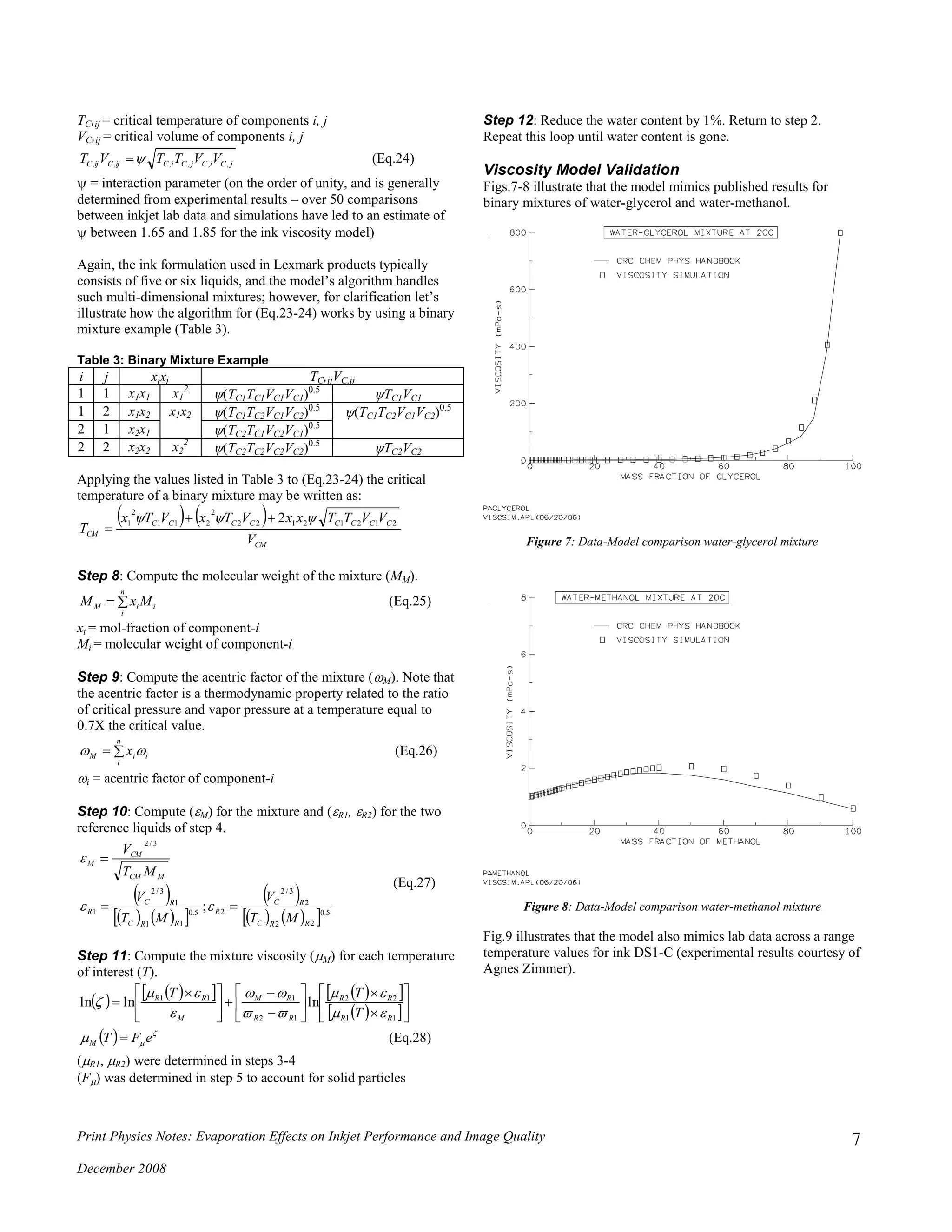
8. Print Physics Notes: Evaporation Effects on Inkjet Performance and Image Quality
December 2008
8
Figure 9: Data-Model comparison DS1-C ink viscosity versus temperature
Finally, Fig.10 illustrates the model results are well correlated over
a range of 57 test cases (the viscosity measurements and
formulations were performed by Agnes Zimmer).
Figure 10: Data-Model correlation over 57 test cases
Ink Property: Mass Diffusivity
The validity of the viscosity model has been established, and
demonstrated to be a relatively accurate means of predicting
viscosity as a function of formulation, temperature and
evaporation. Now can it be used to estimate idle time
performance? No, not just yet - to estimate idle time performance
we also need a predictive means for the evaporation rate. The
evaporation rate is dependent upon knowing the mass diffusivity of
the mixture. That is the topic of this section. It is worth noting that
this is dilemma number two. Predicting the mass diffusivity of a
multi-component liquid mixture is (and historically has been)
problematic.
 Mass diffusivity in many solid materials is generally
predictable due to long range crystal order [19].
 Mass diffusivity in gas is well understood due to kinetic
theory [19].
 Many scientists have worked on developing a kinetic
theory for mass diffusion in liquid:
• Einstein, Stokes, Born, Deybe, Eyring
 Unfortunately, much like the viscosity dilemma, kinetic
theory does not extend to mass diffusion in liquid [7]
 Another complication is that commonly published mass
diffusivity values only hold for binary mixtures at
infinite dilution.
 Mass diffusivity, over a wide solvent-solute range, is
published for only a few binary aqueous mixtures.
 Our ink formulations are not binary, nor are they
infinitely dilute.
 Molecular modeling holds the promise of solving multi-
component mixture diffusivity someday….but published
molecular modeling predictions (USA-ORNL, Spain,
Korea, Norway) show significant deviations from
experiment.
 In the meantime, we must rely on semi-empirical models
to estimate mass diffusivity.
Mass Diffusivity Model
The diffusivity model makes use of the Wilke-Chang method
[7][8]. This is said to be an empirical modification of the Stokes-
Einstein relation.
  6.0
8
104.7
BMIX
AMIX
AB
V
MT
D



 (Eq.29)
DAB = mutual diffusion coefficient (cm2
/s) between components A
and B
TMIX = temperature (K) of the liquid mixture
MIX = viscosity (cP) of the mixture at TMIX
MA = molecular weight of water (g/mol)
VB = molar volume of the non-aqueous ink components (cm3
/mol)
 = association factor of the solvent
[Wilke-Chang recommends ( = 2.6) when the solvent is water]
The Wilke-Chang method is intended for use in binary mixtures.
As mentioned earlier, ink mixtures are not binary. However, they
may be generally classified as mixtures of water (M = 18 g/mol)
and a cocktail of high molecular weight co-solvents (M ~ 100-200
g/mol). So for the purposes of this model, component-A is water
and component-B is treated as a quadratic mixture of the co-
solvents.
Note that the mass diffusion coefficient (DAB) is inversely
proportional to the mixture viscosity. This should be expected
since mass transport in liquids requires the molecules to squeeze
past each other as they move from point(x) to point(x+x). Thus it
is quite natural that there should be a connection between viscosity
and mass diffusivity. Mixture viscosity increases as evaporation
removes water (leaving a higher content of viscous glycols), and a
corresponding DAB reduction is expected.

Diffusivity Model Validation
Table 4 shows an excellent correlation between published DAB
values [10] and (Eq.29) for several binary mixtures.

9. Print Physics Notes: Evaporation Effects on Inkjet Performance and Image Quality
December 2008
9
Table 4: Computed DAB Compared to Reported Experimental
values [10]
Solute in an infinite
dilution of water
T(C)
DAB (10-5
cm2
/s)
Experimental
Value
Wilke-Chang
Equation
Acetone 25 1.28 1.28
Ethanol 25 1.24 1.41
Ethylene glycol 25 1.16 1.28
Glycerol 25 1.06 1.02
Methanol 15 1.28 1.41
1-propanol 15 0.87 0.9
Sucrose 25 0.52 0.58
Cyclohexane 20 0.84 0.83
3-methyl-1-butanol 10 0.69 0.59
Aniline 25 0.91 1.06
Eq.29 does a good job of predicting DAB for binary mixtures that
are infinitely dilute. However, it is known that DAB varies with
viscosity. So it begs the question: If it is known how viscosity
varies as a function of the mixture, can W-C be used to predict DAB
over a wide range of concentrations? This is important to know
because as water evaporates from the ink the water concentration
varies widely. Let us answer this by studying an example in the
literature.
Transport Canada funded a research project to evaluate the
effectiveness of new de-icing fluids [11]. Fundamental to solving
the problem was an understanding of diffusion characteristics of
the candidate mixtures. The University of Quebec measured
diffusion coefficients as part of the project. To validate their
diffusion measurement technique, they first calibrated it against
published values for water-EG mixtures. Their experimental results
along with the values computed with (Eq.29) are shown in Fig.11.
Figure 11: Data-Model correlation for water-EG mixtures
Fig.11 illustrates an important point - mass diffusivity is not a
constant. It varies greatly with water concentration. Any attempt to
simulate evaporation rate and idle time performance must account
for this.
Failing to account for mass diffusivity as a variable can easily
cause an order of magnitude error in the solution of (Eq.19).
Solution Procedure
The groundwork has now been laid, so it is time to apply all of the
teachings to a multi-physics solution.
 Ink Formulation
 Flow Feature Geometry
 Ink Temperature
 Water Evaporation
 Mass Diffusivity
 Viscosity
Ink Simulation Example
The model workspace contains thermodynamic information [Tb,
Tc, Pc, Vc, Zc, Mw,(Tref), (Tamb), Vb, ] for a wide variety of
chemicals. These thermodynamic properties are used, as described
previously, to simulate ink viscosity as a function of temperature
and water loss.
Table 5: Gen1 ink formulation
Component Wt.%
C M Y
DI water 67.79 69.54 69.21
Glycerol 12.5 6 6
Tripropylene glycol 7.5 --- ---
Triethylene glycol 5.5 7 7
1,3-Propanediol --- 8 8
Surfactant 0.75 0.9 0.8
Biocide* 0.13 0.13 0.13
Wax emulsion 0.5 0.5 0.5
Pigment** 4 6 6.5
Dispersant** 1.33 1.93 1.86
*The biocide is ignored in the model because it has a negligible
mol-fraction.
**The pigment and its encapsulating dispersant are considered
solids and are handled with the aforementioned Krieger-Dougherty
equation.
Figure 12: Data-Model correlation for Gen1-Magenta

10. Print Physics Notes: Evaporation Effects on Inkjet Performance and Image Quality
December 2008
10
Figure 13: Mass diffusivity versus viscosity Gen1-Magenta
Fig.12-13 illustrate the simulation results for Gen-1 magenta. Note
the exponential rise in viscosity as ink evaporates from the
mixture. This mimics the actual response of lab data as measured
by Shirish Mulay (Fig. 14).
Figure 14: Lab results – exponential viscosity increase with evaporation
Also note how mass diffusivity plummets as viscosity increases
(Fig 13). If the ink was pure water its diffusivity would be 300
m2
/s, and if the ink contained just 10% water, the remaining, high
viscosity components drive DAB to 8 m2
/s.
To put these values into perspective consider that the mass
diffusivity of moist air at 25C is 25,000,000 m2
/s. That said, the
limiting factor is the diffusivity in the liquid. Once a water
molecule makes it to the air-liquid interface there is no waiting line
to transport it into the free stream. In other words for the special
case of inkjet:
Evaporation of the volatile species generates concentration
gradients in the liquid such that mass transport within the
liquid is rate-limiting.
Finite Element Analysis
Using the finite element method, Fick’s 2nd law can now be
solved. Recall (Eq.19) and the finite element mesh of the mass
diffusion domain.
t
c
y
c
D
yx
c
D
x
WWW






















Fick’s 2nd
Law (Eq.19)
Figure 6: Typical mass diffusion field with evaporative boundary condition
The finite element method is a powerful numerical procedure
that can be applied to a wide variety of application areas. It had its
beginnings in the aerospace industry about 50 years ago, and was
primarily used for structural and solid mechanics problems. It did
not gain wide acceptance until computing power became
ubiquitous (and cheap). Today the finite element method is
commonly used to solve problems in all areas of mathematical
physics. If one can write a set of governing partial differential
equations for the phenomena, it can be solved via the finite
element method. Therefore, it is well suited to the multi-physics
problems so common in inkjet.
There are several excellent books on this topic, and they
should be studied by anyone interested in print physics modeling
[6][12][13]. This section will provide a brief overview of the
numerical procedure that is the finite element method. In this
overview the field variable will be referred to as (). This makes
the discussion generic, applying equally to heat transfer, mass
diffusion, electric field, solid mechanics, etc.
Fig.15 shows the basic 3-node triangular element. The mesh
consists of (N) such elements interconnected at the nodes. The
meshing routine is an exercise in analytical geometry. It will be
covered in a future article.
100% Water
10% Water remaining
In the mixture

11. Print Physics Notes: Evaporation Effects on Inkjet Performance and Image Quality
December 2008
11
Figure 15: Triangular finite element
Diffusive Element Equations
Over the element, variable () is given by:
   
 
   yx
NNN
NNN
mji
mji
m
j
i
mji
e
,variableofvaluesnodal
functionsioninterpolat
)(
















(Eq.30a)
It can be shown that the shape functions are:
























yx
yx
yx
A
N
N
N
mmm
jjj
iii
e
m
j
i



)(
2
1
(Eq.30b)
Where:
areaelement
1
1
1
det2
)(
)(


e
mm
jj
ii
e
A
yx
yx
yx
A
(Eq.30c)













ijmmijjmi
jimimjmii
iiiimmimijmjmii
xxxxxx
yyyyyy
xyyxyxxyxyyx



(Eq.30d)
Since field problems like those described by (Eq.18-19) are often
gradient dependent, it is convenient to write the gradient term as:
 

















y
xg (Eq.30e)
Taking derivatives of (Eq.30a):
 


























































m
j
i
mji
mji
m
j
i
mji
mji
A
y
N
y
N
y
N
x
N
x
N
x
N
g


2
1
In a more compact form the gradient term may be restated as:
     Bg (Eq.30g)
Field problems having the form of (Eq.18-19) have a diffusive
material property associated with them:
 
 
 
B-Aspeciesbetweenydiffusivitmassmutual
0
0
:ydiffusivitisotropicy withdiffusivitmassFor
directionsy)(x,intyconductivithermal,
0
0
:problemferheat transFor the
















AB
AB
AB
MATL
yx
y
x
MATL
D
D
D
D
KK
K
K
D
(Eq.30h)
Field problems having the form of (Eq.18-19) have diffusive-like
and convective-like properties. The diffusive-like term is handled
as:
        
 
elementtheofthickness
equationelementdiffusive
:Where
)(
)(
)()()(



e
e
D
MATL
Teee
D
thk
k
BDBAthkk
(Eq.30i)
Convective Element Equations
The convective terms occur at domain boundaries, as shown in
Fig.16. Since convection is a function of exposed area, the element
equations must take that into account.
   
 
 
  miEXP
mjEXP
jiEXP
e
EXPconve
conv
LL
LL
LL
thkLh
k








































and;
201
000
102
:m)-(iissideelementexposedtheif
and;
210
120
000
:m)-(jissideelementexposedtheif
and;
000
021
012
:j)-(iissideelementexposedtheif
6
)(
)(




(Eq.30j)
hconv = convective coefficient;
- if [ = temperature (T)]; hconv = hc of (Eq.17)
- if [ = concentration (cW)]; hconv = hD/air of (Eq.17a)
LEXP = exposed element length = Li-m in (Fig.16)

12. Print Physics Notes: Evaporation Effects on Inkjet Performance and Image Quality
December 2008
12
Figure 16: Arbitrary mesh showing a convection boundary condition
Global Matrices
The mesh consists of (NNODE) nodes and (NELE) elements. For
each element (Eq.30i) is written, and for elements that have a
convective boundary (Eq.30j) is added to it.
     )()()( e
conv
e
D
e
kkk  (Eq.30k)
The individual element equations are assembled into a global
matrix {K}. Since the finite element method had its roots in
structural mechanics, the {K} matrix is often referred to as the
global stiffness matrix.
Breaking up the domain into an interconnected mesh of finite
elements allows the numerical solution to take the form of
algebraic matrix equations, like (Eq.30m), instead of the often
intractable partial differential equations when applied to complex
geometries and boundary conditions.
         0


FK
t
C (Eq.30m)
 
   
 
(Eq.18)aldifferentipartialFor the
(Eq.19)aldifferentipartialFor the1
211
121
112
12
matrixecapacitancGlobal
matrixstiffnessGlobal
:Where
)()(
)(
1
)(
P
ee
e
NNODE
e
C
Athk
c
cC
K


















(Eq.30n)
For elements with a convective boundary condition:
   
 
 

























0
1
1
2
:(Eq.19)aldifferentipartialFor
0
1
1
2
:(Eq.18)aldifferentipartialFor
matrixforceGlobal
)(
)(
)(
)(
1
)(
AIR
e
EXPDe
e
EXPCe
NNODE
e
thkLWh
f
thkLTh
f
fF

(Eq.30m)
Note (Eq.30m), as shown, is for elements with a convective
boundary along element side i-j. If the convective boundary is on
side j-m the (3 x 1) matrix is [0 1 1]T
. If convection is along side i-
m the (3 x 1) matrix is [1 1 0]T
.
Matrix Equation Solution
Eq.30m may be solved by many numerical techniques. The central
difference method is shown below.
     
     
      FPS
KC
t
P
C
t
KA
OLD 

















2
2
(Eq.30n)
[OLD] = nodal values of the field variable at the last time step
t = time step
To account for convective and fixed boundary conditions, [A] and
[S] must be modified. There are many techniques to do this (e.g.
see Appendix 3 of reference [6]). A convenient mathematical trick
is to identify the node numbers that are affected by fixed and/or
convective conditions. Then multiply the diagonal terms of those
nodes in [A] by a very large number (e.g. 1015
). Next set the
affected nodes of [S] equal to the boundary condition value and
multiply those terms by the same very large number. The set of
equations may now be solved using various matrix reduction
techniques.
     MODMODNEW SA
1
 (Eq.30p)
[NEW] = nodal values of field variable at time (t+t)
[AMOD] [SMOD] are the matrices of (Eq.30n) that have been
modified for fixed and/or convective boundary conditions.
i
j
m
Li-m
j
i m

Free
Stream
Convection Boundary

13. Print Physics Notes: Evaporation Effects on Inkjet Performance and Image Quality
December 2008
13
Because the mesh usually contains thousands of nodes, matrix
inversion is an impractical means of solving (Eq.30p). Matrix
inversion is storage and CPU intensive. The LXK model uses node
renumbering to minimize the bandwidth of the [AMOD] matrix, and
since the matrix is symmetrical, only the upper, non-zero terms,
are stored and manipulated. The details of the bandwidth reduction
method and the rectangular matrix solver algorithm will be
covered in a future article.
After each time step (t), the field variables are laminated
onto a results matrix {}.
 



























nNNODENNODENNODENNODE
n
n
n
tntttttt
,3,2,1,
,32,31,30,3
,23,21,20,2
,13,11,10,1
0 2
For each element, at each time step, there is an associated gradient
as shown in (Eq.30g). Gradients of the field variable are the prime
movers of some flux variable. Flux is the flow rate of some
physical property per unit area. The generic flux over each element
(e) is given by:
     )()()()( eee
MATL
e
BDFlux 
Where:
 
     format.equationmatrixelement,finitein
:andform,equationaldifferentipartialin
)()()( eee
Bg
Grad


In particular, the energy flux in a heat transfer problem (Eq.18) is
given by:
      












 22
)()()()(
ms
Joules
m
Watts
TBDq eee
MATL
e
(Eq.30q)
Similarly for the mass diffusion problem (Eq.19), the mass flux is
given by:
    











 
2
)()()()(
)(
ms
grams
cBDm
e
W
ee
MATL
e
e
 (Eq.30r)
[DMATL] is given by (Eq.30h)
(e)
is the density of the material in the element
To determine the evaporative mass flux leaving the ejector
(Eq.30r) is summed over the elements at the nozzle exit.
Evaporative Flux Exiting an Inkjet Nozzle
The groundwork has now been laid for computing the evaporation
of water vapor from an inkjet ejector and the resultant, transient
viscosity field in the flow features. Reviewing the steps to get to
this point, it was necessary to quantify:
- The thermodynamic properties of moist air
- Boundary layer analysis for (hC, hD) convection coefficients
- Heat and mass diffusion
- Ink viscosity simulation method
- Mass diffusivity (DAB) for multi-component ink mixture
- Finite element analysis overview
Demonstration Example
The example chosen here is the evaporation of water from a
Romulan ejector filled with Puddy2-CMY dye inks. This ink-
ejector combination was chosen because evaporation lab data
exists to check the model veracity. The CMY-flow field is shown
in Fig.17. The K1-K2 flow fields are not shown because those
nozzles were not part of this experiment (they were intentionally
covered with tape so that PM1-mono ink would not confound the
experiment with its clumping, nozzle-blocking tendency). The
Puddy2 ink formulation is shown in Table 6. The simulated
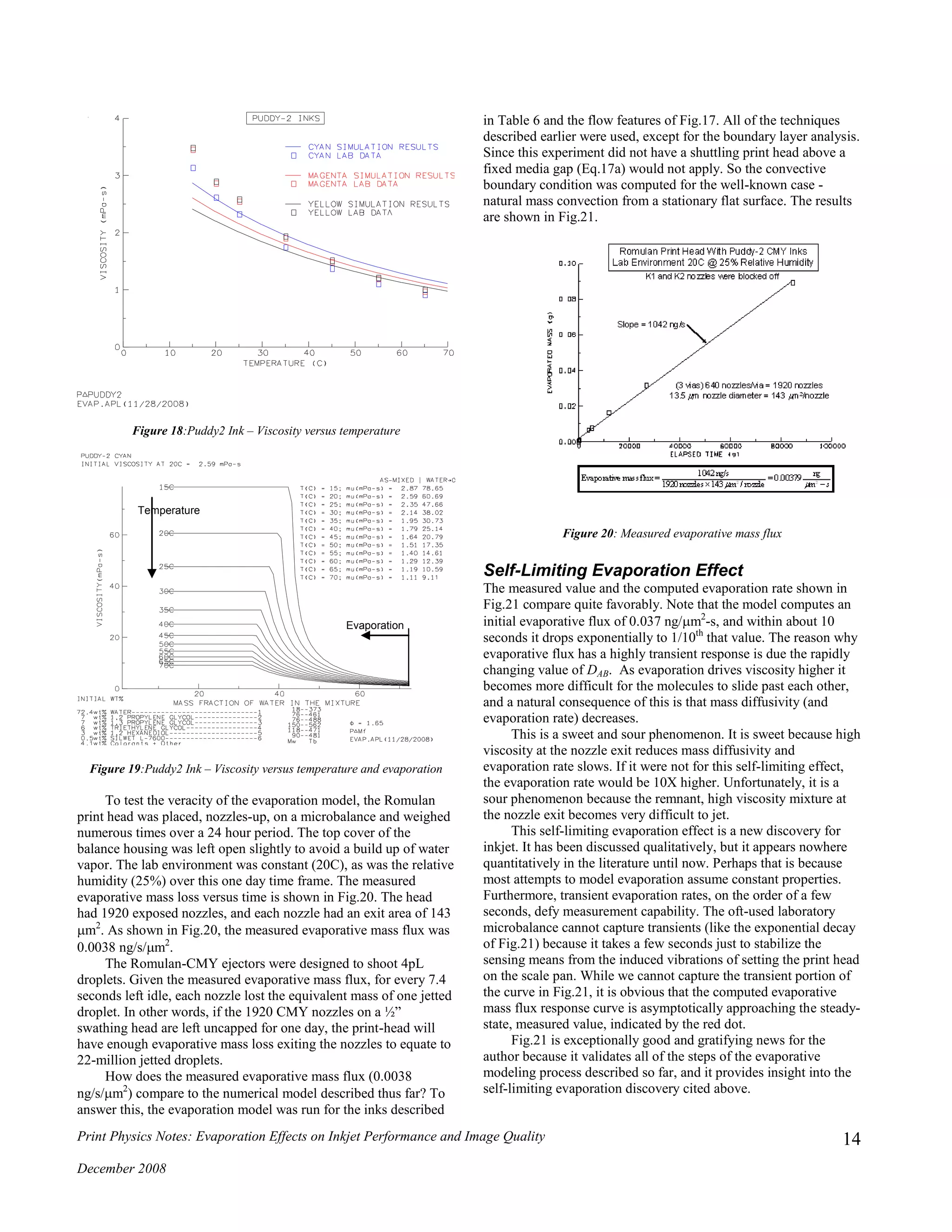
viscosity versus temperature results are shown in Fig.18 along with
the measured values [(T) measurements courtesy of Agnes
Zimmer]. Except at very low temperatures, the model-lab data
comparisons are good for all three inks. Fig.19 shows how
viscosity is expected to vary with temperature and evaporative
mass loss.
Figure 17: Romulan-PINP color ejector
Table 6: Puddy2 ink formulation
Component Wt.%
C M Y
DI water 72.4 72.4 72.3
1,2-propanediol 7.0 --- ---
1,3-propanediol 7.0 6.0 7.0
Triethylene glycol 6.0 --- 6.0
1,2-hexanediol 3.0 3.0 3.0
trimethylolpropane --- 6.0 ---
1,5-pentanediol --- 8.0 ---
Tripropylene glycol --- --- 7.0
Silwet 0.5 0.5 0.5
Biocide 0.1 0.1 0.1
triethanolamine --- --- 0.1
Dye 4.0 4.0 4.0

14. Print Physics Notes: Evaporation Effects on Inkjet Performance and Image Quality
December 2008
14
Figure 18:Puddy2 Ink – Viscosity versus temperature
Figure 19:Puddy2 Ink – Viscosity versus temperature and evaporation
To test the veracity of the evaporation model, the Romulan
print head was placed, nozzles-up, on a microbalance and weighed
numerous times over a 24 hour period. The top cover of the
balance housing was left open slightly to avoid a build up of water
vapor. The lab environment was constant (20C), as was the relative
humidity (25%) over this one day time frame. The measured
evaporative mass loss versus time is shown in Fig.20. The head
had 1920 exposed nozzles, and each nozzle had an exit area of 143
m2
. As shown in Fig.20, the measured evaporative mass flux was
0.0038 ng/s/m2
.
The Romulan-CMY ejectors were designed to shoot 4pL
droplets. Given the measured evaporative mass flux, for every 7.4
seconds left idle, each nozzle lost the equivalent mass of one jetted
droplet. In other words, if the 1920 CMY nozzles on a ½”
swathing head are left uncapped for one day, the print-head will
have enough evaporative mass loss exiting the nozzles to equate to
22-million jetted droplets.
How does the measured evaporative mass flux (0.0038
ng/s/m2
) compare to the numerical model described thus far? To
answer this, the evaporation model was run for the inks described
in Table 6 and the flow features of Fig.17. All of the techniques
described earlier were used, except for the boundary layer analysis.
Since this experiment did not have a shuttling print head above a
fixed media gap (Eq.17a) would not apply. So the convective
boundary condition was computed for the well-known case -
natural mass convection from a stationary flat surface. The results
are shown in Fig.21.
Figure 20: Measured evaporative mass flux
Self-Limiting Evaporation Effect
The measured value and the computed evaporation rate shown in
Fig.21 compare quite favorably. Note that the model computes an
initial evaporative flux of 0.037 ng/m2
-s, and within about 10
seconds it drops exponentially to 1/10th
that value. The reason why
evaporative flux has a highly transient response is due the rapidly
changing value of DAB. As evaporation drives viscosity higher it
becomes more difficult for the molecules to slide past each other,
and a natural consequence of this is that mass diffusivity (and
evaporation rate) decreases.
This is a sweet and sour phenomenon. It is sweet because high
viscosity at the nozzle exit reduces mass diffusivity and
evaporation rate slows. If it were not for this self-limiting effect,
the evaporation rate would be 10X higher. Unfortunately, it is a
sour phenomenon because the remnant, high viscosity mixture at
the nozzle exit becomes very difficult to jet.
This self-limiting evaporation effect is a new discovery for
inkjet. It has been discussed qualitatively, but it appears nowhere
quantitatively in the literature until now. Perhaps that is because
most attempts to model evaporation assume constant properties.
Furthermore, transient evaporation rates, on the order of a few
seconds, defy measurement capability. The oft-used laboratory
microbalance cannot capture transients (like the exponential decay
of Fig.21) because it takes a few seconds just to stabilize the
sensing means from the induced vibrations of setting the print head
on the scale pan. While we cannot capture the transient portion of
the curve in Fig.21, it is obvious that the computed evaporative
mass flux response curve is asymptotically approaching the steady-
state, measured value, indicated by the red dot.
Fig.21 is exceptionally good and gratifying news for the
author because it validates all of the steps of the evaporative
modeling process described so far, and it provides insight into the
self-limiting evaporation discovery cited above.
Evaporation
Temperature

15. Print Physics Notes: Evaporation Effects on Inkjet Performance and Image Quality
December 2008
15
At this point, we can infer the model treats the following correctly:
- The thermodynamic properties of moist air
- Boundary layer analysis for (hC, hD) convection coefficients
- Heat and mass diffusion
- Ink viscosity simulation method
- Mass diffusivity [DAB()] for multi-component ink mixture
- Finite element analysis of the mass diffusion domain
Figure 21: Evaporative mass flux-measured and simulated
Mass Diffusion Field Results
Recall the governing partial differential equation (Eq.19).
Everything is now in place to solve it for any given ejector design,
ink formulation, idle time and environmental condition.
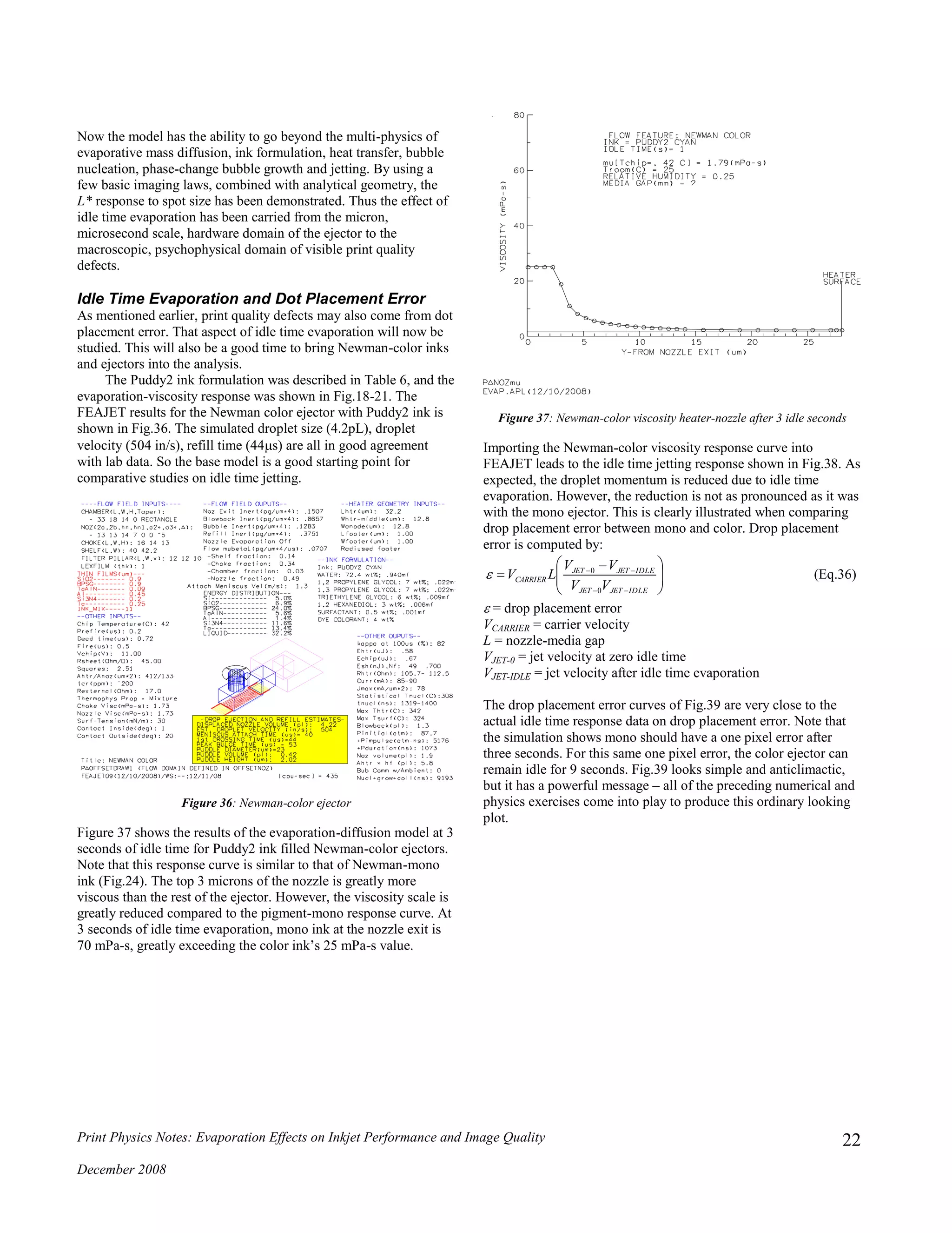
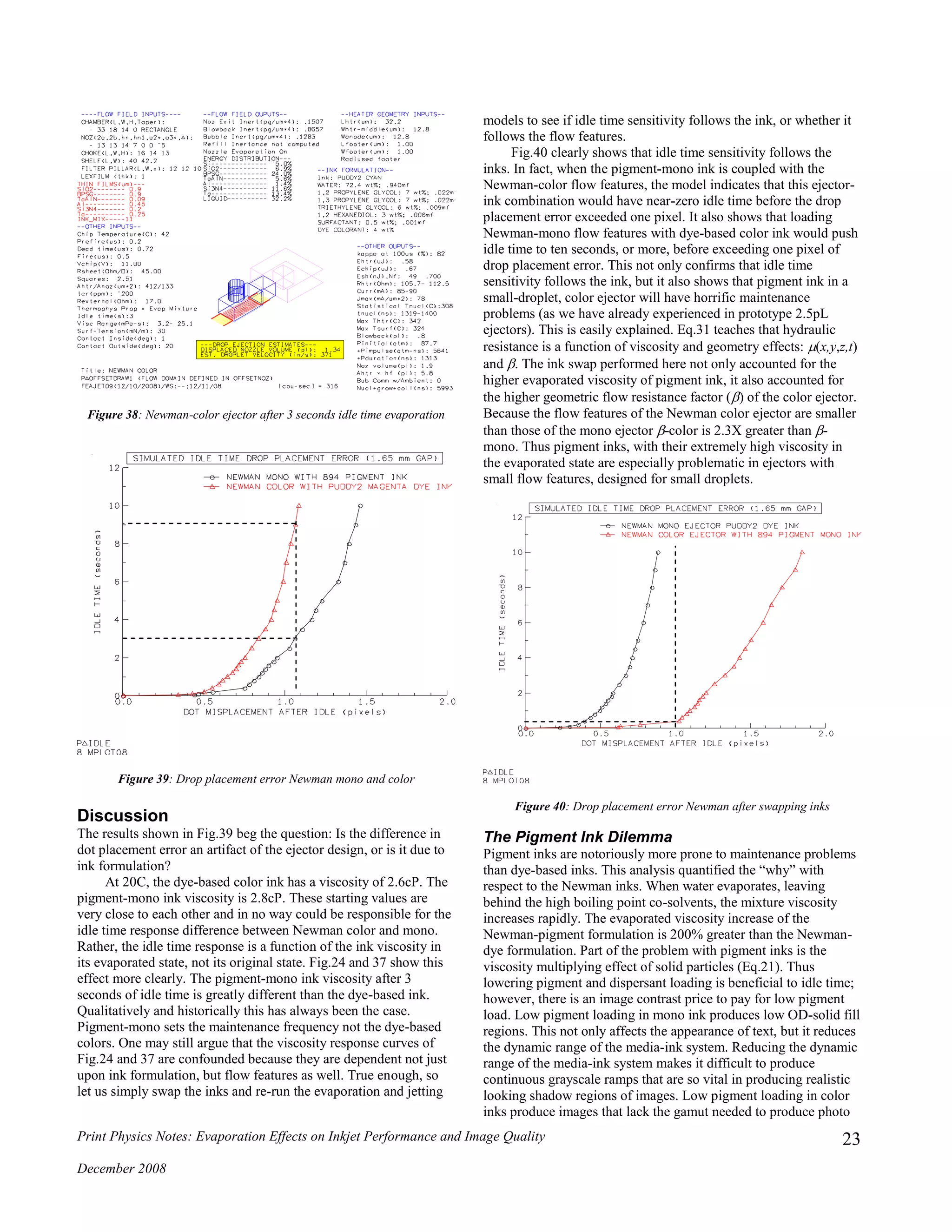
Let us shift focus to Newman-mono. It will be beneficial to
use these teachings to quantitatively show why this ejector-ink
system is more prone to have idle time problems than Newman-
CMY (and Canon-mono).
Fig.22 shows the Newman-mono water concentration field
after just one second of idle time evaporation from a chip held at
42C in an atmosphere of 25C and 25% R.H. Also note the insert in
the upper right corner of Fig.22 showing viscosity versus nozzle
location. According to these results, liquid at the top 2 microns of
the nozzle has a viscosity of 70mPa-s after just one second of idle
time evaporation. That is an increase of 35X over the initial
mixture at 42C.
Recall the earlier comment that HP spits their Edgeline head
every 800 ms because they said substantial changes to
pigment ink properties occur within seconds. Fig.22-23
confirms - substantial changes indeed.
Figure 22: Water concentration after one second of evaporation
Figure 23: Water concentration after ten seconds of evaporation
85,000 s
Evaporative Mass Flux
Experimental Result
0.0038 ng/s-m
2
Simulated evaporative flux

16. Print Physics Notes: Evaporation Effects on Inkjet Performance and Image Quality
December 2008
16
Evaporation Effects on Jetting:
Merging the Models
Fig.I shows the dramatic effect that idle time has on print quality.
After just 3 seconds, the droplets become weak, misdirected and
tiny as evidenced by the poorly formed, wiggly gray line in Fig.I.
The information presented thus far quantifies exactly what happens
to the liquid during those idle seconds – the ink in the nozzle
becomes highly viscous (Fig.24).
The previous discussion focused on the evaporative mass flux
and the resultant impact on ink viscosity. It remains to be shown
how the transient viscosity field affects jetting performance. That
is the topic to be covered in this section – merging the
evaporation/viscosity model with the jetting model.
Figure I: Idle Time Effect
Figure 24: Newman-mono viscosity heater-nozzle after 3 idle seconds
Jetting Model - FEAJET Overview
Over the last two decades, the jetting model has evolved from a
simple heat transfer model into a complex multi-physics ejector
design tool with the following capabilities:
- Current density distribution
- Transient heat transfer
- Bubble nucleation
- Thermal boundary layer in the ink
- Phase change and heat transfer at a moving bubble wall
- Vapor pressure pulse and explosive bubble growth
- Inertance and hydraulic resistance of the flow field
- Outflow from the nozzle and blowback at the choke
- Non-traditional heater shapes
- Thermal stress in the thin films
Now we will add a module to accommodate idle time evaporation
and the resultant effect on jetting.
A typical simulation summary is shown in Fig.25. This particular
set of input variables defines Newman-mono: flow features, ink
formulation, pulse train, electrical properties and heater thin films.
The output variables predicted by the model are on target with the
experimental results. For instance, ejected mass (5.21 ng) and
velocity (454 in/s) are in line with experimental results. Also, the
predicted onset of nucleation (1345-1432 ns) is in agreement with
lab data. Furthermore, the simulation predicts a refill time (first
meniscus crossing) at 50 s – indicating that the maximum fire
frequency is 20 KHz. This too is very much in line with the actual
hardware (within microseconds) because it is known that mono
refills faster than the 18 KHz required.
Having established that the jetting model is a good predictor
of Newman-mono performance, let us use this ejector-ink system
as a test case to illustrate the merged models.
Figure 25: Newman-mono ejector
Hydraulic Resistance
The phase change pressure pulse must overcome inertance and
viscous resistance to accelerate the ink in the ejector. Because ink
density is relatively insensitive to water evaporation, idle time does
not affect inertance. However, idle time evaporation greatly affects
viscous resistance. Therefore, there is no reason to focus on
anything other than the shift of hydraulic resistance as the water
evaporates. Hydraulic resistance may be defined as:

17. Print Physics Notes: Evaporation Effects on Inkjet Performance and Image Quality
December 2008
17
 












dzP
tz
P
HYD 

(Eq.31)
Where:
 
 s/mrateflowvolumetric
)(mfactorresistancehydraulicgeometric
s)-(Paexitnozzle-heaterfromviscositydynamic
nozzle)-(heaterdirection-zin thes/m)-(Pagradientpressure
(Pa)resistancehydraulictoduedroppressure
3
4-










t
z
z
P
PHYD


FEAJET solves for volumetric flow rate by iteration. As the bubble
grows, liquid is converted to water vapor. This phase change
requires energy. The source of the phase-change energy is the
thermal boundary layer in the ink at the onset of nucleation. So
phase-change energy pulled from the thermal boundary layer tends
to cool liquid-vapor interface. Also, at nucleation the temperature
gradient in the thermal boundary layer is on the order of 300
million Kelvin per meter. This gigantic gradient effects rapid
diffusion of thermal energy into the cool region of the ink.
Combining the diffusion effect with the phase-change effect causes
a very rapid cooling of the ink. With the rapid cooling comes a
rapid decrease in the phase-change pressure pulse. The phase-
change pressure pulse and the resultant bubble growth act as a
virtual piston – displacing liquid in the ejector and shooting ink
onto the media. The nature of the explosive phase-change pressure
pulse is seen by comparing Fig.26a and Fig.26b. In both of these
cases the end-point is when the bubble reaches its maximum
displacement, i.e. the onset of bubble collapse. When the pressure
pulse must overcome a highly viscous flow field, the pressure
pulse is spent more quickly. For example, the 3 second idle time
case (Fig.26a) expends its pressure pulse in about 1.6 s, while the
0 second idle time pressure pulse (Fig.26b) lasts about 3.6 s.
These pressure-temperature response curves are a function of how
hard the bubble has to work to move liquid. There is a fixed
amount of available energy in the thermal boundary layer for
phase-change. So when the viscous resistance is high, the pressure
pulse is quickly dissipated.
Figure 26a: Newman-mono phase change pressure pulse after 3 seconds of
idle time evaporation
Figure 26b: Newman-mono phase change pressure pulse after 0 seconds of
idle time evaporation
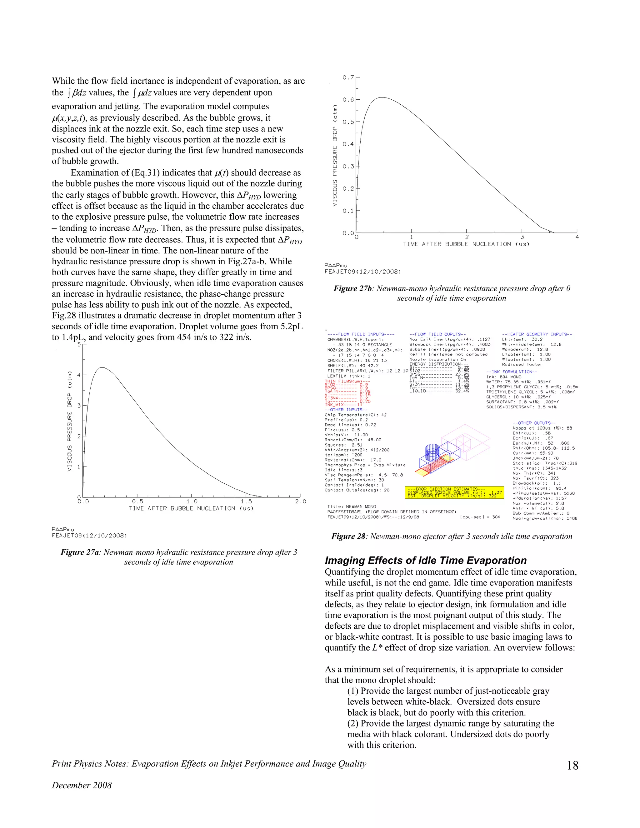
Fig.26 illustrates the effect of PHYD. As for the other terms in
(Eq.31), the evaluation of  dz can be problematic because, like
many MEMS flow structures, inkjet ejectors are non-circular. This
presents a problem for micro-flow fields, but a solution
methodology was derived and published in 2007 [14]. Instead of
repeating those teachings here, interested parties may consult [14].
The result for the Newman-mono flow features  dz is given by:
0.00579 (m-3
) shelf region
0.00677 (m-3
) choke region
0.00133 (m-3
) chamber region
0.00884 (m-3
) nozzle region

18. Print Physics Notes: Evaporation Effects on Inkjet Performance and Image Quality
December 2008
18
While the flow field inertance is independent of evaporation, as are
the  dz values, the  dz values are very dependent upon
evaporation and jetting. The evaporation model computes
(x,y,z,t), as previously described. As the bubble grows, it
displaces ink at the nozzle exit. So, each time step uses a new
viscosity field. The highly viscous portion at the nozzle exit is
pushed out of the ejector during the first few hundred nanoseconds
of bubble growth.
Examination of (Eq.31) indicates that (t) should decrease as
the bubble pushes the more viscous liquid out of the nozzle during
the early stages of bubble growth. However, this PHYD lowering
effect is offset because as the liquid in the chamber accelerates due
to the explosive pressure pulse, the volumetric flow rate increases
– tending to increase PHYD. Then, as the pressure pulse dissipates,
the volumetric flow rate decreases. Thus, it is expected that PHYD
should be non-linear in time. The non-linear nature of the
hydraulic resistance pressure drop is shown in Fig.27a-b. While
both curves have the same shape, they differ greatly in time and
pressure magnitude. Obviously, when idle time evaporation causes
an increase in hydraulic resistance, the phase-change pressure
pulse has less ability to push ink out of the nozzle. As expected,
Fig.28 illustrates a dramatic decrease in droplet momentum after 3
seconds of idle time evaporation. Droplet volume goes from 5.2pL
to 1.4pL, and velocity goes from 454 in/s to 322 in/s.
Figure 27a: Newman-mono hydraulic resistance pressure drop after 3
seconds of idle time evaporation
Figure 27b: Newman-mono hydraulic resistance pressure drop after 0
seconds of idle time evaporation
.
Figure 28: Newman-mono ejector after 3 seconds idle time evaporation
Imaging Effects of Idle Time Evaporation
Quantifying the droplet momentum effect of idle time evaporation,
while useful, is not the end game. Idle time evaporation manifests
itself as print quality defects. Quantifying these print quality
defects, as they relate to ejector design, ink formulation and idle
time evaporation is the most poignant output of this study. The
defects are due to droplet misplacement and visible shifts in color,
or black-white contrast. It is possible to use basic imaging laws to
quantify the L* effect of drop size variation. An overview follows:
As a minimum set of requirements, it is appropriate to consider
that the mono droplet should:
(1) Provide the largest number of just-noticeable gray
levels between white-black. Oversized dots ensure
black is black, but do poorly with this criterion.
(2) Provide the largest dynamic range by saturating the
media with black colorant. Undersized dots do poorly
with this criterion.

19. Print Physics Notes: Evaporation Effects on Inkjet Performance and Image Quality
December 2008
19
Criteria (1) and (2) compete with each other. This suggests that the
mono droplet characteristics need to be considered carefully. So it
begs the question, can we mathematically describe the transition
from white to black? To answer that, let us begin with the
relationship between area coverage and digital grayscale levels (0-
255).
The relationship between area coverage and digital grayscale
begins with an exercise in analytical geometry. Localized regions
of the image can be made white, black, or any discrete gray level
in between, but individual pixels can only be white or black. This
fact suggests that grayscale imaging involves the art of distributing
errors. The art of how individual droplets are laid down to
minimize visible patterns is constantly being improved. For the
purpose of this analysis the Floyd-Steinberg error diffusion pattern
will be applied to determine the grayscale dot patterns. For F-S
error diffusion, Fig.29 shows the pixel overlap types. For each of
the 10 types, the region of interest includes a 3 x 3 box of pixels.
The center pixel (crosshatched) is the one being considered. It is
surrounded by pixels that have already been considered (the solid
colored circles and rectangles). When an inkjet device is
considering whether to print the center pixel in this box it may, or
may not print the dot. This binary decision creates an error because
these choices amount to a pixel grayscale of 0 or 255. If the region
under consideration is supposed to be a gray level in between, an
error is created. The Floyd-Steinberg error diffusion algorithm
distributes this error to the pixels to the right and below, as they
have yet to be considered. The incremental area generated by
printing the center, crosshatched dot is a function of the
surrounding neighbors that have already been considered. For the
Floyd-Steinberg error diffusion algorithm, there are 10 unique
overlap types to consider for computing the incremental area of the
center pixel. The analytical geometry functions are made
applicable to any pixel resolution by normalizing the dot size to the
pixel size (Eq.32).
)0.20(;
sizepixel
diameterSpot
 FF (Eq.32)
There are many error diffusion techniques. They all have the same
goal – grayscale reproduction while minimizing visible pattern
artifacts. We are simply using this particular error diffusion
method to estimate the incremental printed area as the digital
grayscale level goes from 0-255. We are not using it to study
pattern visibility and Fourier analysis. Surprisingly, the Floyd-
Steinberg error diffusion algorithm produces nearly the same
incremental area coverage as the antiquated Bayer 16 x 16 halftone
algorithm, and it will be shown later that it well describes the
incremental area function of the halftone algorithm used in
Rushmore. Fig.30 shows the F-S results: incremental area coverage
as a function of digital halftone level for (F) values from 0.5 to 2.0.
Type A
Type B
Type C
Type D
Type E
Type F
Type G
Type H
Blank neighbor from
previous scan
Filled neighbor from
previous scan
Current pixel
being printed
Error diffusion
neighbor
x
y
Scan directions
Pel
Size
Spot
Diameter sizePel
diameterSpot
F
Type J
Type K
Analytical geometry functions are derived to
determine the dot fill area for each overlap type
(F < 2.0)
Computing The Area Fill Fraction By Analyzing
Pixel Overlap Types In An Error Diffusion Pattern
Thisismathematicallytractable
withanalyticalgeometry
Figure 29: Pixel overlap types
Pel
Size
Spot
Diameter sizePel
diameterSpot
F
F
=
1.4
F
=
2.0
Figure 30: Area coverage as a function of F and digital halftone level
The blank page has a reflective luminance Ymax. The solid fill
region of the page has a reflective luminance Ymin. Between Ymax
and Ymin the gray levels exist. An 8-bit white-black transition has
256 digital levels. A representative (0-255) gray ladder is shown in
Fig.31. This curve shows the measured values of reflective
luminance (Y) for a spot size value of (F = 1.74).
Figure 31a: Measured reflectance for pigment-mono ink with normalized
spot size F = 1.74
Ymax
Blank page
Ymin
Solid Fill
For F = 1.74

20. Print Physics Notes: Evaporation Effects on Inkjet Performance and Image Quality
December 2008
20
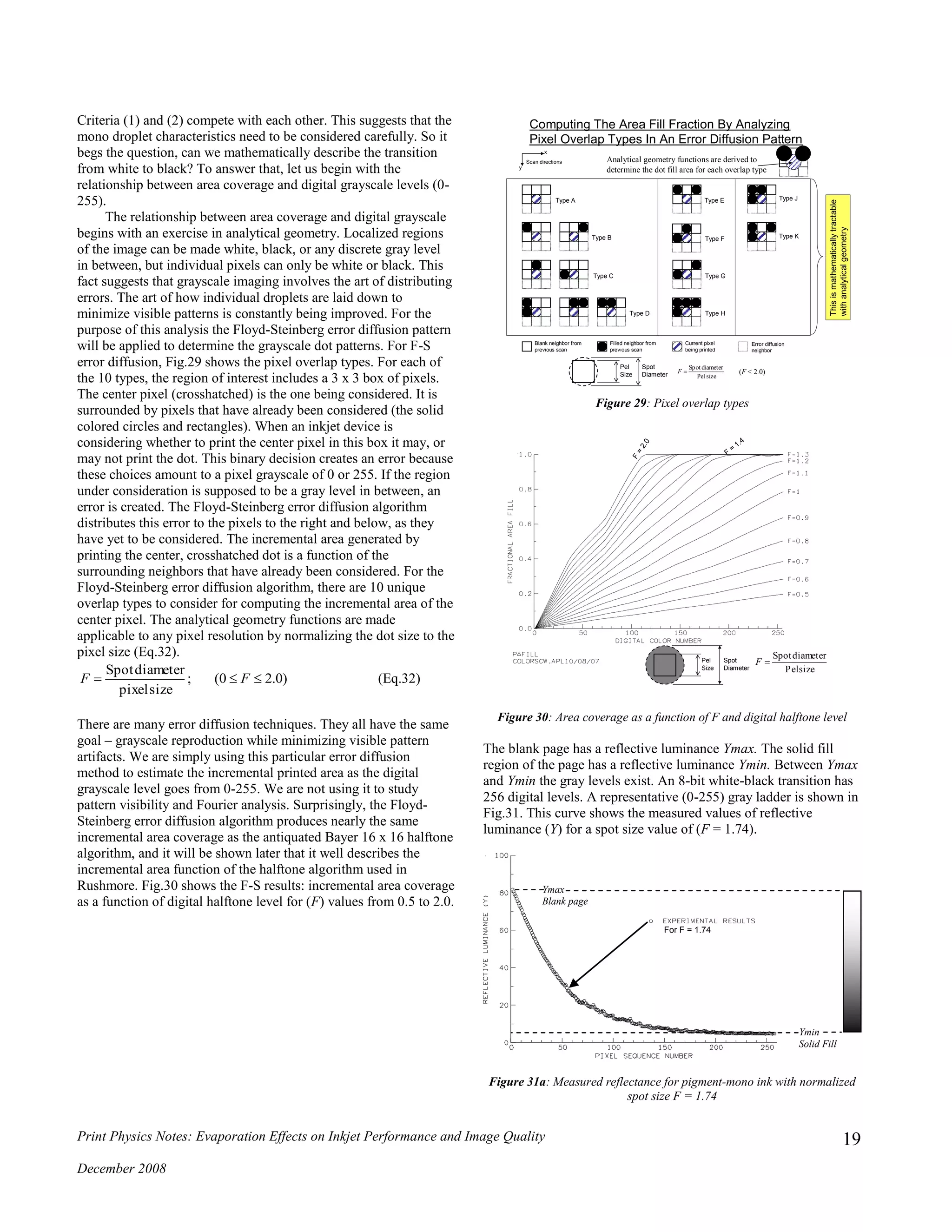
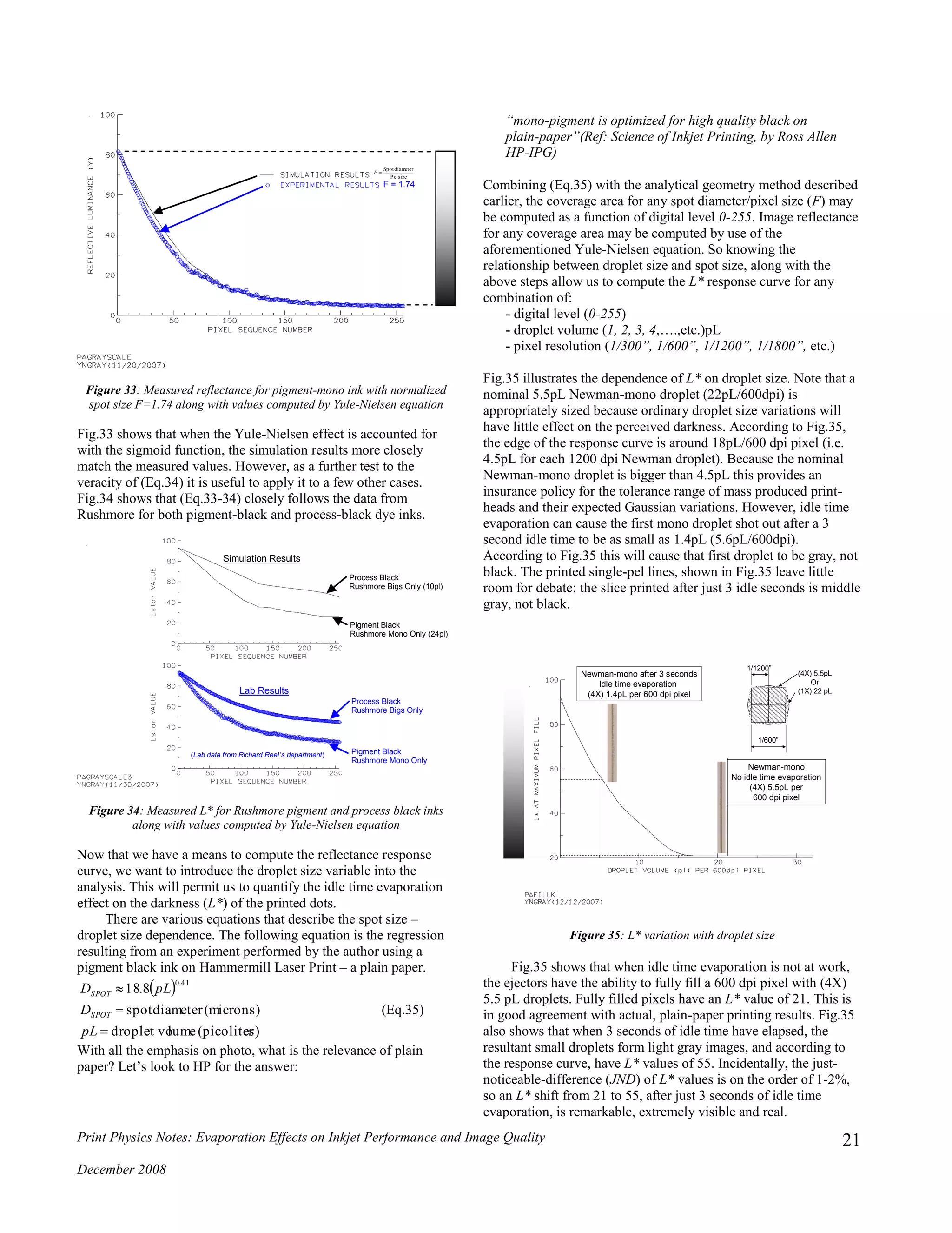
The cira-1936 Murray-Davies equation relates area coverage to
reflective luminance. Unfortunately, as shown in Fig.31b, it does a
poor job of matching the lab data over much of the experimental
space.
Figure 31b: Measured reflectance for pigment-mono ink with normalized
spot size F = 1.74 along with values computed by Murray-Davies equation
So the obvious solution relating luminance and grayscale, based
simply upon incremental dot area coverage, is the wrong one.
However, it is interesting to note that the Murray-Davies equation
matches the experimental data in the solidly filled region, but it
does a poor job in the regime where dot coverage is low. This
observation provides a clue to the source of the discrepancy. The
discrepancy is explained by examining what happens to the light
when it enters the non-dot regions (Fig.32). Because the media
scatters light in the non-dot regions, some of the diffused light
exits in the dot regions. Thus sparsely placed dots absorb more
light than their area alone would suggest. This discovery is
attributed to Yule and Nielsen (1957) [15].
Figure 32: Internal light reflections in the non-dot regions of the media
tcoefficienNielsen-Yule
fractioncoveragearea
fillsolidofdensitydottheofdensity
paperblankofdensity
density
1011log
:isequationNielsen-YuletheofformdensityThe
10



















n
c
DD
D
D
cnDD
a
Pd
P
n
dD
aP
(Eq.33)
 















 
16
100
116*
:by*familiarmorethetoconvertedthenisformereflectancThe
0.10;10
:byereflectanctoconvertedisformdensityThe
3/1
Y
L
L
RR D
DP and Dd are known from densitometry measurements (solid fill
and blank paper). Coverage area (ca) is computed by analytical
geometry. What value is to be placed upon (n)?
Physical arguments behind the derivation of (Eq.33) suggest
that n is contained within the range of 1 to 2. Furthermore, it can
be shown that as the dot coverage (ca) goes to unity, n goes to
unity. In other words, when there is little to no non-dot area there
is no need to account for the scattering effect shown in Fig.32. The
literature abounds with various means of estimating (n). Since
there is no general agreement within the image science community,
the sigmoid function proposed here (Eq.34) is both easy and
reasonable.
 
0.05factorsteepnessslope
ntransitiobatheofpoint-mid
)0.10(fractioncoveragearea
1.0regionsfill-solidin thefactorNielsen-Yule
2.0regionsdot-nonin thefactorNielsen-Yule
exp1
0
0










 



w
x
xcx
b
a
w
xx
ba
an
a
(Eq.34)
Figure 33: Sigmoid function for Yule-Nielsen factor (n)
  
RY
RcRR daP
100
11


R = image reflectivity
Rp = paper reflectance
Rd= dot reflectance
ca = area coverage fraction
Ymax
Blank page
Ymin
Solid Fill
F = 1.74
DotDot
Dot
Media
Light Rays
The media scatters the light entering the non-dot regions.
Some of the scattered light is absorbed by nearby dots.
The sigmoid function is used in this analysis to
determine n as a function of area coverage*
n  2
n  1

21. Print Physics Notes: Evaporation Effects on Inkjet Performance and Image Quality
December 2008
21
Figure 33: Measured reflectance for pigment-mono ink with normalized
spot size F=1.74 along with values computed by Yule-Nielsen equation
Fig.33 shows that when the Yule-Nielsen effect is accounted for
with the sigmoid function, the simulation results more closely
match the measured values. However, as a further test to the
veracity of (Eq.34) it is useful to apply it to a few other cases.
Fig.34 shows that (Eq.33-34) closely follows the data from
Rushmore for both pigment-black and process-black dye inks.
Figure 34: Measured L* for Rushmore pigment and process black inks
along with values computed by Yule-Nielsen equation
Now that we have a means to compute the reflectance response
curve, we want to introduce the droplet size variable into the
analysis. This will permit us to quantify the idle time evaporation
effect on the darkness (L*) of the printed dots.
There are various equations that describe the spot size –
droplet size dependence. The following equation is the regression
resulting from an experiment performed by the author using a
pigment black ink on Hammermill Laser Print – a plain paper.
 
s)(picoliterlumedroplet vo
(microns)diameterspot
8.18
41.0



pL
D
pLD
SPOT
SPOT
(Eq.35)
With all the emphasis on photo, what is the relevance of plain
paper? Let’s look to HP for the answer:
“mono-pigment is optimized for high quality black on
plain-paper”(Ref: Science of Inkjet Printing, by Ross Allen
HP-IPG)
Combining (Eq.35) with the analytical geometry method described
earlier, the coverage area for any spot diameter/pixel size (F) may
be computed as a function of digital level 0-255. Image reflectance
for any coverage area may be computed by use of the
aforementioned Yule-Nielsen equation. So knowing the
relationship between droplet size and spot size, along with the
above steps allow us to compute the L* response curve for any
combination of:
- digital level (0-255)
- droplet volume (1, 2, 3, 4,….,etc.)pL
- pixel resolution (1/300”, 1/600”, 1/1200”, 1/1800”, etc.)
Fig.35 illustrates the dependence of L* on droplet size. Note that a
nominal 5.5pL Newman-mono droplet (22pL/600dpi) is
appropriately sized because ordinary droplet size variations will
have little effect on the perceived darkness. According to Fig.35,
the edge of the response curve is around 18pL/600 dpi pixel (i.e.
4.5pL for each 1200 dpi Newman droplet). Because the nominal
Newman-mono droplet is bigger than 4.5pL this provides an
insurance policy for the tolerance range of mass produced print-
heads and their expected Gaussian variations. However, idle time
evaporation can cause the first mono droplet shot out after a 3
second idle time to be as small as 1.4pL (5.6pL/600dpi).
According to Fig.35 this will cause that first droplet to be gray, not
black. The printed single-pel lines, shown in Fig.35 leave little
room for debate: the slice printed after just 3 idle seconds is middle
gray, not black.
1/600”
1/1200”
(4X) 5.5pL
Or
(1X) 22 pL
Newman-mono
No idle time evaporation
(4X) 5.5pL per
600 dpi pixel
Newman-mono after 3 seconds
Idle time evaporation
(4X) 1.4pL per 600 dpi pixel
Figure 35: L* variation with droplet size
Fig.35 shows that when idle time evaporation is not at work,
the ejectors have the ability to fully fill a 600 dpi pixel with (4X)
5.5 pL droplets. Fully filled pixels have an L* value of 21. This is
in good agreement with actual, plain-paper printing results. Fig.35
also shows that when 3 seconds of idle time have elapsed, the
resultant small droplets form light gray images, and according to
the response curve, have L* values of 55. Incidentally, the just-
noticeable-difference (JND) of L* values is on the order of 1-2%,
so an L* shift from 21 to 55, after just 3 seconds of idle time
evaporation, is remarkable, extremely visible and real.
F = 1.74
sizePel
diameterSpot
F
Process Black
Rushmore Bigs Only
Pigment Black
Rushmore Mono Only
Lab Results
Simulation Results
Process Black
Rushmore Bigs Only (10pl)
Pigment Black
Rushmore Mono Only (24pl)
(Lab data from Richard Reel’s department)

22. Print Physics Notes: Evaporation Effects on Inkjet Performance and Image Quality
December 2008
22
Now the model has the ability to go beyond the multi-physics of
evaporative mass diffusion, ink formulation, heat transfer, bubble
nucleation, phase-change bubble growth and jetting. By using a
few basic imaging laws, combined with analytical geometry, the
L* response to spot size has been demonstrated. Thus the effect of
idle time evaporation has been carried from the micron,
microsecond scale, hardware domain of the ejector to the
macroscopic, psychophysical domain of visible print quality
defects.
Idle Time Evaporation and Dot Placement Error
As mentioned earlier, print quality defects may also come from dot
placement error. That aspect of idle time evaporation will now be
studied. This will also be a good time to bring Newman-color inks
and ejectors into the analysis.
The Puddy2 ink formulation was described in Table 6, and the
evaporation-viscosity response was shown in Fig.18-21. The
FEAJET results for the Newman color ejector with Puddy2 ink is
shown in Fig.36. The simulated droplet size (4.2pL), droplet
velocity (504 in/s), refill time (44s) are all in good agreement
with lab data. So the base model is a good starting point for
comparative studies on idle time jetting.
Figure 36: Newman-color ejector
Figure 37 shows the results of the evaporation-diffusion model at 3
seconds of idle time for Puddy2 ink filled Newman-color ejectors.
Note that this response curve is similar to that of Newman-mono
ink (Fig.24). The top 3 microns of the nozzle is greatly more
viscous than the rest of the ejector. However, the viscosity scale is
greatly reduced compared to the pigment-mono response curve. At
3 seconds of idle time evaporation, mono ink at the nozzle exit is
70 mPa-s, greatly exceeding the color ink’s 25 mPa-s value.
Figure 37: Newman-color viscosity heater-nozzle after 3 idle seconds
Importing the Newman-color viscosity response curve into
FEAJET leads to the idle time jetting response shown in Fig.38. As
expected, the droplet momentum is reduced due to idle time
evaporation. However, the reduction is not as pronounced as it was
with the mono ejector. This is clearly illustrated when comparing
drop placement error between mono and color. Drop placement
error is computed by:







 



IDLEJETJET
IDLEJETJET
CARRIER
VV
VV
LV
0
0
 (Eq.36)
 = drop placement error
VCARRIER = carrier velocity
L = nozzle-media gap
VJET-0 = jet velocity at zero idle time
VJET-IDLE = jet velocity after idle time evaporation
The drop placement error curves of Fig.39 are very close to the
actual idle time response data on drop placement error. Note that
the simulation shows mono should have a one pixel error after
three seconds. For this same one pixel error, the color ejector can
remain idle for 9 seconds. Fig.39 looks simple and anticlimactic,
but it has a powerful message – all of the preceding numerical and
physics exercises come into play to produce this ordinary looking
plot.

23. Print Physics Notes: Evaporation Effects on Inkjet Performance and Image Quality
December 2008
23
Figure 38: Newman-color ejector after 3 seconds idle time evaporation
Figure 39: Drop placement error Newman mono and color
Discussion
The results shown in Fig.39 beg the question: Is the difference in
dot placement error an artifact of the ejector design, or is it due to
ink formulation?
At 20C, the dye-based color ink has a viscosity of 2.6cP. The
pigment-mono ink viscosity is 2.8cP. These starting values are
very close to each other and in no way could be responsible for the
idle time response difference between Newman color and mono.
Rather, the idle time response is a function of the ink viscosity in
its evaporated state, not its original state. Fig.24 and 37 show this
effect more clearly. The pigment-mono ink viscosity after 3
seconds of idle time is greatly different than the dye-based ink.
Qualitatively and historically this has always been the case.
Pigment-mono sets the maintenance frequency not the dye-based
colors. One may still argue that the viscosity response curves of
Fig.24 and 37 are confounded because they are dependent not just
upon ink formulation, but flow features as well. True enough, so
let us simply swap the inks and re-run the evaporation and jetting
models to see if idle time sensitivity follows the ink, or whether it
follows the flow features.
Fig.40 clearly shows that idle time sensitivity follows the
inks. In fact, when the pigment-mono ink is coupled with the
Newman-color flow features, the model indicates that this ejector-
ink combination would have near-zero idle time before the drop
placement error exceeded one pixel. It also shows that loading
Newman-mono flow features with dye-based color ink would push
idle time to ten seconds, or more, before exceeding one pixel of
drop placement error. This not only confirms that idle time
sensitivity follows the ink, but it also shows that pigment ink in a
small-droplet, color ejector will have horrific maintenance
problems (as we have already experienced in prototype 2.5pL
ejectors). This is easily explained. Eq.31 teaches that hydraulic
resistance is a function of viscosity and geometry effects: (x,y,z,t)
and . The ink swap performed here not only accounted for the
higher evaporated viscosity of pigment ink, it also accounted for
the higher geometric flow resistance factor () of the color ejector.
Because the flow features of the Newman color ejector are smaller
than those of the mono ejector -color is 2.3X greater than -
mono. Thus pigment inks, with their extremely high viscosity in
the evaporated state are especially problematic in ejectors with
small flow features, designed for small droplets.
Figure 40: Drop placement error Newman after swapping inks
The Pigment Ink Dilemma
Pigment inks are notoriously more prone to maintenance problems
than dye-based inks. This analysis quantified the “why” with
respect to the Newman inks. When water evaporates, leaving
behind the high boiling point co-solvents, the mixture viscosity
increases rapidly. The evaporated viscosity increase of the
Newman-pigment formulation is 200% greater than the Newman-
dye formulation. Part of the problem with pigment inks is the
viscosity multiplying effect of solid particles (Eq.21). Thus
lowering pigment and dispersant loading is beneficial to idle time;
however, there is an image contrast price to pay for low pigment
load. Low pigment loading in mono ink produces low OD-solid fill
regions. This not only affects the appearance of text, but it reduces
the dynamic range of the media-ink system. Reducing the dynamic
range of the media-ink system makes it difficult to produce
continuous grayscale ramps that are so vital in producing realistic
looking shadow regions of images. Low pigment loading in color
inks produce images that lack the gamut needed to produce photo

24. Print Physics Notes: Evaporation Effects on Inkjet Performance and Image Quality
December 2008
24
quality. For example, to satisfy photo-centric imaging scientists,
the Gen1-pigment color formulations had between 6-6.5 wt.%
colorant to achieve the gamut obtained with 4 wt.% dye
formulations. The Gen1-pigment colors also used a polymeric
dispersant that consumed another 1.9 wt.% of the mix (typically in
the industry, pigment-dispersant ratios are about 15:4). Because the
dispersants attach themselves to the pigment particle, the charged
particle shell is physically larger than the dry pigment particle
itself. This effect is illustrated as (D) in Fig.41. That said, when
polymeric dispersants are used in conjunction with pigment
particles, they both go into the Krieger-Dougherty equation, and
the solid volume fraction increases – increasing the viscosity
multiplier of Eq.21.
Pigment Particle Kinetics
The solids account for some of the pigment-dye viscosity
difference. The other part of the issue is that the remnant co-
solvent blend used in pigment formulations are very often more
viscous than those used in the dye formulation. This slows the
pigment retreat as water evaporates – a good thing. Charged
pigment particles seek water to balance the electrostatic field
formed by the double charge layer surrounding them. When
evaporation leaves a humectant-rich, water-poor mixture in the
nozzle, the pigment particles retreat to the water-rich region of the
ink via.
Pigment retreat is a form of electro-kinetics. If a charged
particle is accelerated with respect to the surrounding fluid when
an electric field is applied, the particle kinetics are defined as
electrophoresis. If the fluid moves under the influence of an
electric field, the flow is defined as electro-osmotic. Observations
of pigment particle retreat show that the particles move thru a
stationary liquid, thus the kinetics of pigment retreat is a form of
electrophoresis. When an electric field is placed across a pigment
loaded ink, electrophoretic flow occurs. This is easily seen when
an anode-cathode probe pair is placed in the ink because pigment
particles travel towards one of the probes. The source of the
electric field in capillary electrophoresis may be anode-cathode
pairs as often used in bioMEMS applications [18] (DNA micro-
arrays, Lab-on-chip, hemoglobin electrophoresis, protein analysis,
etc.). Or, the electric field source may be due to ionic and pH
gradients that come about from evaporation driven concentration
gradients of water in the ejector.
Figure 41: Charge field around an electrophoretic particle
Fig.41 shows the double charge layer surrounding a particle. Under
the influence of an electric field, the electrophoretic velocity is
[17]:
Ev L
EP 







0
(Eq.37)
vEP = electrophoretic velocity
0 = zeta potential = f(chemistry, pH, temperature)
L = dielectric constant of the liquid
 = viscosity
E = electric field strength (Volt/m)
If (vEP) is large, the pigment retreat is fast, and the ejected droplets
lack colorant. Pigment retreat is a serious problem – what good is a
jettable ink formulation if the first few droplets have no colorant
due to pigment retreat. Pigment particles move more slowly thru a
high viscosity mixture. Note in (Eq.37), electrophoretic velocity is
inversely proportional to viscosity.
So there is a particle-kinetics benefit to using more viscous
co-solvents in pigment inks. If co-solvents are chosen such that
the mixture has low viscosity in the evaporated state, the idle time
jetting may be unimpeded, but the ejected droplet will have low
colorant loading because the low viscosity mixture allows rapid,
electrophoretic transport of pigment particles away from the water-
poor nozzle towards the water-rich ink via. Yet, if the co-solvents
are viscous enough to slow the pigment kinetics, they form a
highly viscous plug, a few microns long, that impedes jetting.
There may be a middle ground between dye-based and
pigment-based formulations that offer the best set of tradeoffs
between image permanence, gamut, pigment retreat
(electrophoresis) and idle time jetting. If so, the viscosity response
curves will likely lie between those of Fig.19 (dye) and Fig.42
(pigment).
Figure 19:Puddy2-dye-ink – Viscosity versus temperature and evaporation

25. Print Physics Notes: Evaporation Effects on Inkjet Performance and Image Quality
December 2008
25
Figure 42:894 Pigment-mono ink – Viscosity versus temperature and
evaporation
Epson Pigment-Color Ink
In Lexmark’s market segments, the nearly universal rule is that
mono ink is pigment (with droplets >> 4pL) and color is dye-based
(with droplets < 4pL). An exception to this rule is Epson. With
their piezo-electric technology they have chosen to incorporate
pigment-color inks. Let’s examine their formulation to see if they
have discovered the magic where image permanence, gamut
pigment particle kinetics and idle time jetting live happily in
unison. Tab.7 (courtesy of Agnes Zimmer) lists our best analytical
chemistry estimate of the Epson C88 Pigment-Magenta ink
formulation. Fig.43 shows the viscosity response curves of this ink.
The simulation shows that this ink has a room temperature (20C)
viscosity of 4.36cP. Epson, on their MSDS [16], reports this ink
having a viscosity less than 5cP, so the simulation results agree
with the published information. The Epson C88 pigment color
viscosity response curves look nearly identical to the Gen1-
pigment magenta results shown earlier in Fig.12. The Gen1
pigment-CMY formulations were simply horrible from an idle time
viewpoint. That said, it is clear that Epson may have a pigment ink
formulation for image permanence and probably not prone to
pigment retreat; however, the enormous viscosity in the evaporated
state means that the C88 formulation has no magical idle time
properties.
Table 7: Epson C88 pigment-magenta ink formulation
Component Wt.%
2-pyrollidone 3.2
Glycerol 12.6
Triethylene glycol mono butyl ether 2.5
Trimethyol propane 4.3
1,2-Hexanediol 2
Water 70
Colorant – dispersant load Bal (5.4)
Figure 43:Epson C88 Pigment-color ink – Viscosity versus temperature
and evaporation
HP Pigment-Mono Ink
The mono-pigment formulation from HP is shown in Table 8
(courtesy Agnes Zimmer), and its viscosity response curves are
shown in Fig.44. According to the simulation the HP-mono ink
should have a viscosity of 3.5cP at 20C. This agrees very well with
the experimental value of 3.3cP at 22C. It is interesting to note that
the HP pigment mono formulation has much lower viscosity in the
evaporated state than all other pigment inks examined in this
document. In the evaporated state the HP pigment mono ink looks
more like Puddy2-dye inks than 894-mono pigment, Gen1-color
pigment and Epson-color pigment. This does not imply that HP has
found the magic spot where pigment inks are optimized, but it
clearly shows that they understand the issues and the importance of
not allowing the evaporated state viscosity to leap up to values
greater than dye-based inks.
Table 8: HP88 pigment-mono ink formulation
Component Wt.%
2-pyrollidone 18.8
2-methyl-1,3-propanediol 2
Tetraethylene glycol 2
Water 71.3
Colorant – dispersant load Bal (6)

26. Print Physics Notes: Evaporation Effects on Inkjet Performance and Image Quality
December 2008
26
Figure 44:HP88 Pigment-mono ink – Viscosity versus temperature and
evaporation
Canon Pigment-mono Ejector
One last set of simulations is worth a short discussion here to
quantify how the ejector design knobs may be used to enable
robust idle time with pigment ink. Let us examine the pros and
cons of Canon’s mono ejector. This is an interesting design point
because it is a throwback to where Lexmark ejectors were a decade
ago – 600 dpi, large droplet. To isolate the effect of this ejector
design, allowing direct comparison to Newman-mono, let us fill it
with 894-pigment mono ink. Fig.45 shows the simulation summary
for this design point. Canon does not publish the size of their mono
droplets; however, it is quite likely that the predicted value is
correct because at 23pL per 600dpi pixel, this ejector shoots a very
good droplet size according to Lexmark criteria (and Fig.35).
Figure 45: Canon mono-pigment 600 dpi ejector
Fig.46 shows that the Canon ejector with pigment mono ink is far
less prone than Newman to produce pixel-sized drop placement
errors even after 10 seconds of idle. It is more likely that Canon-
mono idle time is set by loss of colorant due to droplet size
reduction, as shown in Fig.47. This plot clearly illustrates the value
of a 600dpi ejector when pigment-mono inks are used. After 5
seconds of idle, the Canon droplet size falls to about 14pL. At
14pL the first droplet shot is in the vicinity of one JND- L* unit (a
just noticeable difference of reflective luminance).
The primary use of pigment mono is for text. At 600 dpi, text
is about as good as it needs to be. There is really no need for
pigment mono in images as long as the process black is dark
enough to ensure high contrast and dynamic range. By coupling a
600dpi mono ejector that shoots 22+pL, with 1200 dpi, multi-level
color ejectors (1.5 – 4.5pL), Canon has chosen to design their
mono-pigment ejector for text and the color-dye ejectors for
images. In so doing, they avoid the idle time issues that are so
problematic when one tries to use pigment inks in conjunction with
high resolution (1200dpi) and small droplets (<5pL).
As mentioned at the outset of this report, idle time physics is
not about using models to find bulletproof, optimized designs –
rather it is about using models to identify the proper tradeoffs. In
Canon’s case, the tradeoffs were system architecture decisions, not
just tweaks to hardware designs.
Figure 46: Drop placement error Newman and Canon mono
Figure 47: L* variation due to idle time Newman and Canon mono

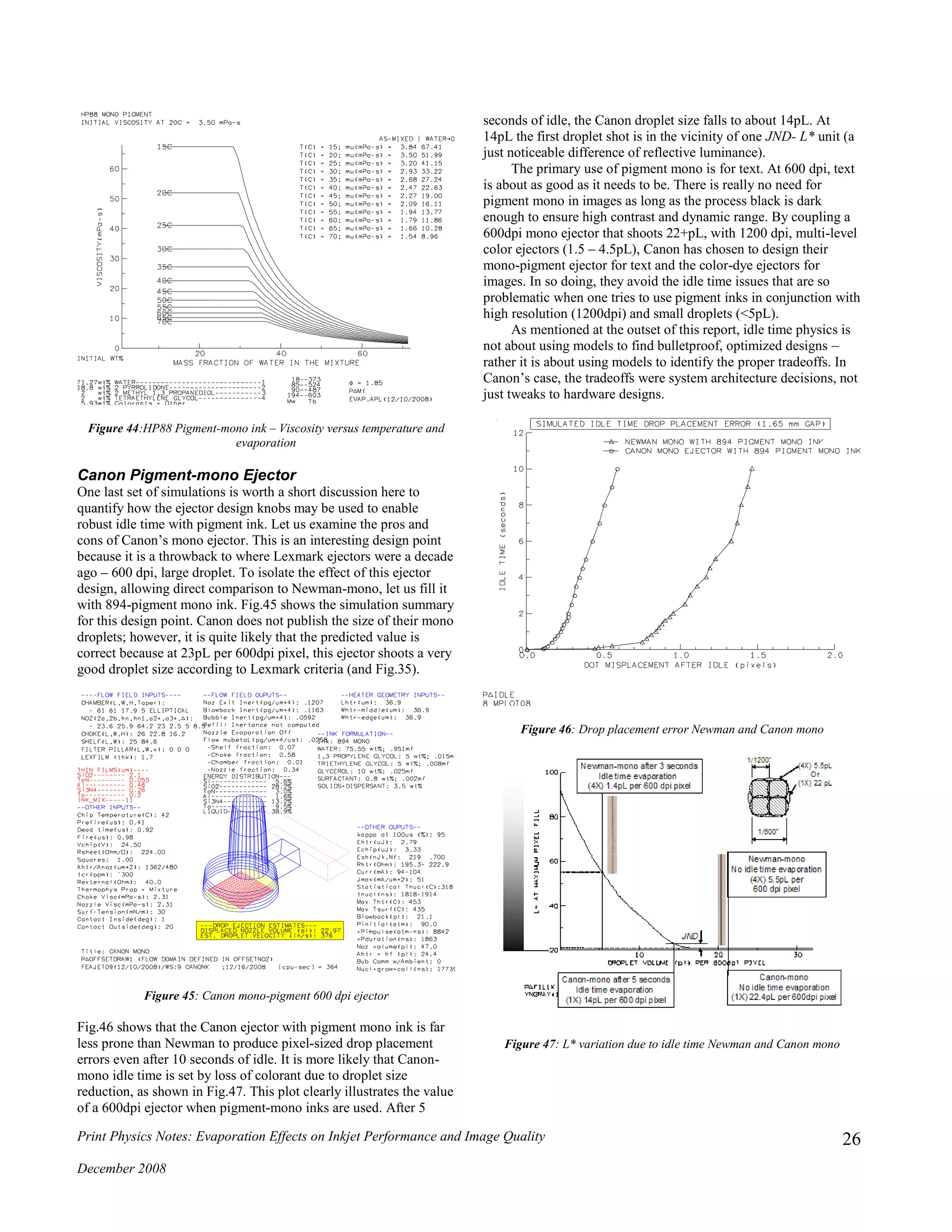
27. Print Physics Notes: Evaporation Effects on Inkjet Performance and Image Quality
December 2008
27
Conclusions
Idle time brings to mind idyllic Summer scenes of sipping lemonade
on the porch swing. However, like most things inkjet, idle time is
anything but an easy, mindless exercise. This document has shown
that to quantify inkjet idle time one needs to make use of multiple
areas of science; ink formulations, heat and mass diffusion on both
sides of the liquid-air interface, thermodynamic interactions
between moist air and water, the thermo-hydrodynamics of jetting
and some aspects of image science. Even with all these fields
covered there are gaps in the unknown – for instance the
quantitative electro-kinetics of pigment retreat. There are always
gaps in knowledge, but that does not mean what is known is
irrelevant. This article has shown consistent veracity between
experimental results and simulations. Also, the analysis has shown
the self-limiting characteristic of idle time evaporation from a
quantitative viewpoint. Furthermore, it has shown direct cause and
effect between idle time evaporation and the resultant print quality
defects due to L* variations and drop placement error. As mixed
viscosity is important – indeed the ejector flow features are designed
and tuned to this value. However, this analysis clearly shows that
viscosity in the evaporated state is the dominant idle time lever.
Idle time has always been a topic of great concern and debate,
but it never got beyond the qualitative and empirical realms. For the
first time in nearly two decades of inkjet development at Lexmark,
we are now poised to start speaking of idle time issues and tradeoffs
quantitatively.
References
[1] Ross Allen, HP Scaleable Print Technology, 30th
Global Inkjet Printing
Conf., Prague, Czech Rep., (2007).
[2] Beverly, Clint & Fletcher, Evaporation rates of structured and non-
structured liquid mixtures, PCCP, 2, (2000).
[3] J.L. Threlkeld, Thermal Environmental Engineering, 2nd
ed., Prentice-
Hall, Inc., London, (1970).
[4] T. Kusuda, Humidity and Moisture, Vol. 1, (1965).
[5] J.P. Holman, Heat Transfer, McGraw-Hill, New York, (1972).
[6] L.J. Segerlind, Applied Finite Element Analysis, Wiley & Sons, New
York, (1976).
[7] Poling, Prausnitz & O’Connell, The Properties of Gases and Liquids,
McGraw-Hill, New York, (2000)
[8] Bird, Stewart & Lightfoot, Transport Phenomena, Wiley & Sons, New
York, (1976).
[9] V.P. Carey, Liquid-Vapor Phase Change Phenomena, Hemisphere
Publ., Washington, (1992).
[10] D.R. Lide (ed.), Handbook of Chemistry and Physics, 84th
Ed., CRC
Press, Boca Raton, (2003).
[11] Louchez, Zouzou, Liu’ & Sasseville, Modeling of Water Diffusion in
Ground Aircraft De/anti-icing Fluids for Numerical Prediction of
Laboratory Holdover Time, Transportation Development Centre, Montreal,
Quebec, (1997).
[12] D.L. Logan, A First Course in the Finite Element Method, PWS-Kent,
Boston, (1986).
[13] K.H. Huebner, The Finite Element Method for Engineers, Wiley &
Sons, New York, (1975).
[14] R.W. Cornell, Using Solid Mechanics to Evaluate the Capillary and
Viscous Behavior on Non-circular Tube Shapes, Proc. IS&T-NIP23,
(2007).
[15] J.A.C. Yule & W.J. Nielsen, The Penetration of Light into Paper and
its Effect on Halftone Reproduction, Proc TAGA, (1951).
[16] Epson product information sheet PIS T060320, Ver. 3.51 (08/2005).
[17] Geschke, Klank & Tellemann, Microsystem Engineering of Lab-on-a-
Chip Devices, Wiley-VCH, (2004).
[18] S.S. Saliterman, Fundamentals of BioMEMEMS and Medical
Microdevices, SPIE Press, (2006).
[19] W. Jost, Diffusion in Solids, Liquids and Gases, Academic Press, New
York, (1960).