The document discusses flowmetering steam. It begins by quoting Lord Kelvin about the importance of measurement. Many businesses now recognize the value of energy cost accounting, conservation, and monitoring techniques using tools like flowmetering. Steam is difficult to measure accurately. Flowmeters designed for liquids and gases don't always work well for steam. The document then discusses fundamentals of fluid mechanics including density, viscosity, Reynolds number, and flow regimes as they relate to measuring steam flow. Accurately measuring steam use allows optimizing plant efficiency and energy efficiency through monitoring steam demand and identifying major steam users.

1. The Steam and Condensate Loop 4.1.1
Fluids and Flow Module 4.1Block 4 Flowmetering
Module 4.1
Fluids and Flow
SC-GCM-43CMIssue3©Copyright2007Spirax-SarcoLimited

2. The Steam and Condensate Loop4.1.2
Fluids and Flow Module 4.1Block 4 Flowmetering
Introduction
‘When you can measure what you are speaking about and express it in
numbers, you know something about it; but when you cannot measure it,
when you cannot express it in numbers, your knowledge
is of a meagre and unsatisfactory kind’.
William Thomson (Lord Kelvin) 1824 - 1907
Many industrial and commercial businesses have now recognised the value of:
o Energy cost accounting.
o Energy conservation.
o Monitoring and targeting techniques.
These tools enable greater energy efficiency.
Steam is not the easiest media to measure. The objective of this Block is to achieve a greater
understanding of the requirements to enable the accurate and reliable measurement of steam
flowrate.
Most flowmeters currently available to measure the flow of steam have been designed for measuring
the flow of various liquids and gases. Very few have been developed specifically for measuring
the flow of steam.
Spirax Sarco wishes to thank the EEBPP (Energy Efficiency Best Practice Programme) of ETSU
for contributing to some parts of this Block.
Fundamentals and basic data of
Fluid and Flow
Why measure steam?
Steam flowmeters cannot be evaluated in the same way as other items of energy saving equipment
or energy saving schemes. The steam flowmeter is an essential tool for good steam housekeeping.
It provides the knowledge of steam usage and cost which is vital to an efficiently operated plant
or building. The main benefits for using steam flowmetering include:
o Plant efficiency.
o Energy efficiency.
o Process control.
o Costing and custody.
Plant efficiency
A good steam flowmeter will indicate the flowrate of steam to a plant item over the full range of
its operation, i.e. from when machinery is switched off to when plant is loaded to capacity. By
analysing the relationship between steam flow and production, optimum working practices can
be determined.
The flowmeter will also show the deterioration of plant over time, allowing optimum plant cleaning
or replacement to be carried out.
The flowmeter may also be used to:
o Track steam demand and changing trends.
o Establish peak steam usage times.
o Identify sections or items of plant that are major steam users.
This may lead to changes in production methods to ensure economical steam usage. It can also
reduce problems associated with peak loads on the boiler plant.

3. The Steam and Condensate Loop 4.1.3
Fluids and Flow Module 4.1Block 4 Flowmetering
Energy efficiency
Steam flowmeters can be used to monitor the results of energy saving schemes and to compare
the efficiency of one piece of plant with another.
Process control
The output signal from a proper steam flowmetering system can be used to control the quantity
of steam being supplied to a process, and indicate that it is at the correct temperature and
pressure. Also, by monitoring the rate of increase of flow at start-up, a steam flowmeter can be
used in conjunction with a control valve to provide a slow warm-up function.
Costing and custody
Steam flowmeters can measure steam usage (and thus steam cost) either centrally or at individual
user points. Steam can be costed as a raw material at various stages of the production process
thus allowing the true cost of individual product lines to be calculated.
To understand flowmetering, it might be useful to delve into some basic theory on fluid
mechanics, the characteristics of the fluid to be metered, and the way in which it travels through
pipework systems.
Fluid characteristics
Every fluid has a unique set of characteristics, including:
o Density.
o Dynamic viscosity.
o Kinematic viscosity.
Density
This has already been discussed in Block 2, Steam Engineering Principles and Heat Transfer,
however, because of its importance, relevant points are repeated here.
Density (r) defines the mass (m) per unit volume (V) of a substance (see Equation 2.1.2).
Equation 2.1.2

4. Hh††Ã€Ãxt9r†v‡’à Ã2ÃW‚yˆ€rÃWÀ TƒrpvsvpÉ‚yˆ€rà J
U
Y
Steam tables will usually provide the specific volume (vg ) of steam at various pressures/
temperatures, and is defined as the volume per unit mass:
W‚yˆ€rÃW
TƒrpvsvpÉ‚yˆ€rà Ã2À xt
Hh††Ã€
JY
From this it can be seen that density (r) is the inverse of specific volume (vg):
U9r†v‡’à 2Ãxt €
TƒrpvsvpÉ‚yˆ€rÃ
JY
The density of both saturated water and saturated steam vary with temperature. This is illustrated
in Figure 4.1.1.

5. The Steam and Condensate Loop4.1.4
Fluids and Flow Module 4.1Block 4 Flowmetering
Fig. 4.1.1 The density (r) of saturated water (rf) and saturated steam (rg) at various temperatures
Dynamic viscosity
This is the internal property that a fluid possesses which resists flow. If a fluid has a high viscosity
(e.g. heavy oil) it strongly resists flow. Also, a highly viscous fluid will require more energy to
push it through a pipe than a fluid with a low viscosity.
There are a number of ways of measuring viscosity, including attaching a torque wrench to a
paddle and twisting it in the fluid, or measuring how quickly a fluid pours through an orifice.
A simple school laboratory experiment clearly demonstrates viscosity and the units used:
A sphere is allowed to fall through a fluid under the influence of gravity. The measurement of the
distance (d) through which the sphere falls, and the time (t) taken to fall, are used to determine
the velocity (u).
The following equation is then used to determine the dynamic viscosity:
Equation 4.1.1
!Ã ÃtÃ…
9’h€vpÉv†p‚†v‡’à 2
(È
'U
P
0
700
50 100 150 200 250 300
800
900
1000
Density(r)kg/m³
Temperature (°C)
Saturated water
0
10
20
30
40
50
0 50 100 150 200 250 300
Density(r)kg/m³
Temperature (°C)
Saturated steam
Where:
µ = Absolute (or dynamic) viscosity (Pa s)
Dr = Difference in density between the sphere and the liquid (kg /m3)
g = Acceleration due to gravity (9.81 m/s2)
r = Radius of sphere (m)
u =
Note: The density of saturated steam increases with temperature (it is a gas, and is compressible) whilst the
density of saturated water decreases with temperature (it is a liquid which expands).
§ ·
¨ ¸
© ¹
qÃÃ9v†‡hprƃur…rÃshyy†Ã€
Wry‚pv‡’Ã
‡ÃÃUv€rÇhxrÃ‡‚ÃshyyÆrp‚q†

6. The Steam and Condensate Loop 4.1.5
Fluids and Flow Module 4.1Block 4 Flowmetering
There are three important notes to make:
1. The result of Equation 4.1.1 is termed the absolute or dynamic viscosity of the fluid and is
measured in pascal seconds. Dynamic viscosity is also expressed as ‘viscous force’.
2. The physical elements of the equation give a resultant in kg/m, however, the constants
(2 and 9) take into account both experimental data and the conversion of units to pascal
seconds (Pa s).
3. Some publications give values for absolute viscosity or dynamic viscosity in centipoise (cP),
e.g.: 1 cP = 10-3
Pa s
Example 4.1.1
It takes 0.7 seconds for a 20 mm diameter steel (density 7800 kg/m3) ball to fall 1 metre through
oil at 20°C (density = 920 kg/m3).
Determine the viscosity where:
Dr = Difference in density between the sphere (7 800) and the liquid (920) = 6 880 kg/m3
g = Acceleration due to gravity = 9.81 m/s2
r = Radius of sphere = 0.01 m
u = Velocity = 1.43 m/s

8. !Ã ÃtÃ…
9’h€vpÉv†p‚†v‡’à — 2
(È
!ÃÑÃÃ%Ã''ÃÑÃÃ(' ÃÑÃÃ
9’h€vpÉv†p‚†v‡’à — 2 Ã2à $Ã
(ÃÑÃà #
'
QhÆ
U
q
Ã2Ã
‡
§ ·
¨ ¸
© ¹
0 50 100 150 200 250 300
0
500
1000
1500
2 000
Temperature (°C)
Saturated water
0
5
10
15
20
50 100 150 200 250 300
Temperature (°C)
Saturated steam
Dynamicviscosity(µ)x10-6
PasDynamicviscosity(µ)x10-6
Pas
Fig. 4.1.2 The dynamic viscosity of saturated water (mf) and saturated steam (mg) at various temperatures
Note: The values for saturated water decrease with temperature, whilst those for saturated steam increase with temperature.
Values for the dynamic viscosity of saturated steam and water at various temperatures are given
in steam tables, and can be seen plotted in Figure 4.1.2.

9. The Steam and Condensate Loop4.1.6
Fluids and Flow Module 4.1Block 4 Flowmetering
(!ÑÃÃ!ÃÑÃÃ
$
HSr’‚yq†Ãˆ€ir…ÃS 2 2Ãà Ã$!
From looking at the above Reynolds number it can be seen that the flow is in the laminar region
(see Figure 4.1.7).
Equation 4.1.3
Reynolds number (Re)
The factors introduced above all have an effect on fluid flow in pipes. They are all drawn
together in one dimensionless quantity to express the characteristics of flow, i.e. the
Reynolds number (Re).
ÈÃ9
Sr’‚yq†Ãˆ€ir…ÃS 2
—
H
U
Where:
r = Density (kg /m3)
u = Mean velocity in the pipe (m/s)
D = Internal pipe diameter (m)
µ = Dynamic viscosity (Pa s)
Analysis of the equation will show that all the units cancel, and Reynolds number (Re) is therefore
dimensionless.
Evaluating the Reynolds relationship:
o For a particular fluid, if the velocity is low, the resultant Reynolds number is low.
o If another fluid with a similar density, but with a higher dynamic viscosity is transported through
the same pipe at the same velocity, the Reynolds number is reduced.
o For a given system where the pipe size, the dynamic viscosity (and by implication,
temperature) remain constant, the Reynolds number is directly proportional to velocity.
Example 4.1.3
The fluid used in Examples 4.1.1 and 4.1.2 is pumped at 20 m/s through a 100 mm bore pipe.
Determine the Reynolds number (Re) by using Equation 4.1.3 where: r = 920 kg /m3
µ = 1.05 Pa s
Equation 4.1.3
ÈÃ9
Sr’‚yq†Ãˆ€ir…ÃS 2
—
H
U
Kinematic viscosity
This expresses the relationship between absolute (or dynamic) viscosity and the density of the fluid
(see Equation 4.1.2).
Where:
Kinematic viscosity is in centistokes
Dynamic viscosity is in Pa s
Density is in kg/m3
Example 4.1.2
In Example 4.1.1, the density of the oil is given to be 920 kg /m3 - Now determine the kinematic
viscosity:
$ÑÃ
Fvr€h‡vpÉv†p‚†v‡’à 2à à à #Ãpr‡v†‡‚xr†ÃpT‡
(!
Q
Equation 4.1.2
9’h€vpÉv†p‚†v‡’à Ñà Fvr€h‡vpÉv†p‚†v‡’à 2 9r†v‡’Ã
P
Q
U

10. The Steam and Condensate Loop 4.1.7
Fluids and Flow Module 4.1Block 4 Flowmetering
Fig. 4.1.3 Velocity profile ignoring viscosity and friction
Fig. 4.1.4 Velocity profile with viscosity and friction
However, this is very much an ideal case and, in practice, viscosity affects the flowrate of the fluid
and works together with the pipe friction to further decrease the flowrate of the fluid near the
pipe wall. This is clearly illustrated in Figure 4.1.4:
At low Reynolds numbers (2 300 and below) flow is termed ‘laminar’, that is, all motion occurs
along the axis of the pipe. Under these conditions the friction of the fluid against the pipe wall
means that the highest fluid velocity will occur at the centre of the pipe (see Figure 4.1.5).
Fig. 4.1.5 Parabolic flow profile
Flow
Flow
Flow
Flow regimes
If the effects of viscosity and pipe friction are ignored, a fluid would travel through a pipe in a
uniform velocity across the diameter of the pipe. The ‘velocity profile’ would appear as shown in
Figure 4.1.3:

11. The Steam and Condensate Loop4.1.8
Fluids and Flow Module 4.1Block 4 Flowmetering
As the velocity increases, and the Reynolds number exceeds 2300, the flow becomes increasingly
turbulent with more and more eddy currents, until at Reynolds number 10 000 the flow is
completely turbulent (see Figure 4.1.6).
Saturated steam, in common with most fluids, is transported through pipes in the ‘turbulent
flow’ region.
Fig. 4.1.7 Reynolds number
Turbulent flow region
(Re: above 10 000)
Transition flow region
(Re: between 2300 - 10000)
Laminar flow region
(Re: between 100 - 2300)
Flow
Fig. 4.1.6 Turbulent flow profile
Stagnation

12. The Steam and Condensate Loop 4.1.9
Fluids and Flow Module 4.1Block 4 Flowmetering
The examples shown in Figures 4.1.3 to 4.1.7 are useful in that they provide an understanding
of fluid characteristics within pipes; however, the objective of the Steam and Condensate Loop
Book is to provide specific information regarding saturated steam and water (or condensate).
Whilst these are two phases of the same fluid, their characteristics are entirely different. This has
been demonstrated in the above Sections regarding Absolute Viscosity (m) and Density (r).
The following information, therefore, is specifically relevant to saturated steam systems.
Example 4.1.4
A 100 mm pipework system transports saturated steam at 10 bar g at an average velocity of 25 m/s.
Determine the Reynolds number.
The following data is available from comprehensive steam tables:
Tsat at 10 bar g = 184°C
Density (r ) = 5.64 kg/m³
Dynamic viscosity of steam (µ) at 184°C = 15.2 x 10-6 Pa s
Equation 4.1.3
ÈÃ9
Sr’‚yq†Ãˆ€ir…ÃS 2
—
H
U
Where:
r = Density = 5.64 kg/m3
u = Mean velocity in the pipe = 25 m/s
D = Internal pipe diameter = 100 mm = 0.1 m
µ = Dynamic viscosity = 15.2 x 10-6 Pa s
$%#ÃÑÃÃ!$ÃÑÃÃ
S
$!ÃÑÃÃ
H
Re = 927 631 = 0.9 x 106
o If the Reynolds number (Re) in a saturated steam system is less than 10 000 (104) the flow
may be laminar or transitional.
Under laminar flow conditions, the pressure drop is directly proportional to flowrate.
o If the Reynolds number (Re) is greater than 10 000 (104) the flow regime is turbulent.
Under these conditions the pressure drop is proportional to the square root of the flow.
o For accurate steam flowmetering, consistent conditions are essential, and for saturated steam
systems it is usual to specify the minimum Reynolds number (Re) as 1 x 105 = 100000.
o At the opposite end of the scale, when the Reynolds number (Re) exceeds 1 x 106, the head
losses due to friction within the pipework become significant, and this is specified as the
maximum.

13. The Steam and Condensate Loop4.1.10
Fluids and Flow Module 4.1Block 4 Flowmetering
ÃÃÃÃÃ$%#ÃÑÃÈÃÑÃà ÃÃÃÃÃ
Ã
$!ÃÑÃÃ
ÃÃÑÃà ÃÑÃà $!ÃÑÃÃ
$%#ÃÑÃÃ
H
S à 2 ÑÃ
ˆ 2 !%($À †
Volumetric flowrate may be determined using Equation 4.1.4:
Equation 4.1.4„ Ã6ÈY
Equation 4.1.5
T
T
Y
Y
P
J
Equation 4.1.6
6È
„
‰
P
J
Example 4.1.5
Based on the information given above, determine the maximum and minimum flowrates for
turbulent flow with saturated steam at 10 bar g in a 100 mm bore pipeline.
Equation 4.1.3
ÈÃ9
Sr’‚yq†Ãˆ€ir…ÃS 2
—
H
U
Where:
r = Density = 5.64 kg/m3
u = Mean velocity in the pipe (To be determined) m/s
D = Internal pipe diameter = 100 mm (0.1 m)
µ = Dynamic viscosity = 15.2 x 10-6 Pa s
For minimum turbulent flow, Re of 1 x 105 should be considered:
Ã2à Ã2à À xt
$%#
§ ·
¨ ¸
© ¹
JY
Where:
qv = Volume flow (m3/s)
A = Cross sectional area of the pipe (m2)
u = Velocity (m/s)
Mass flowrate may be determined using Equations 4.1.5 and 4.1.6:
Where:
qm = Mass flow (kg/s)
qv = Volume flow (m3/s)
vg = Specific volume (m3/kg)
Equation 4.1.6 is derived by combining Equations 4.1.4 and 4.1.5:
Where:
qm = Mass flow (kg/s)
A = Cross sectional area of the pipe (m2)
u = Velocity (m/s)
vg = Specific volume (m3/kg)

14. The Steam and Condensate Loop 4.1.11
Fluids and Flow Module 4.1Block 4 Flowmetering
Returning to Example 4.1.5, and inserting values into Equation 4.1.6:
S
S
§ ·
¨ ¸
¨ ¸
© ¹
6È 9
„ ÃÃÃà ur…rÃ6Ã2à Ã
‰ #
Ã9 È
„
#É
ÃÑÃà ÃÑÃÃ!%($
Ãà !ÃxtÆ
#ÃÑÃÃ
$%#ÃÑÃÈÃÑÃÃ
S
$!ÃÑÃÃ
ÃÑÃà ÑÃà $!ÃÑÃÃ
$%#ÃÑÃÃ
„
P
J
P
J
P
H
„ #ÃxtÃu
ÑÃ
ˆ 2 !%($À†
S
S
S
6È
‰
Ã9 È
„
#É
ÃÑÃà ÃÑÃÃ!%($
Ãà !ÃxtÆ
#ÃÑÃÃ
P
J
P
J
P
ò
„ #ÃxtÃu
Similarly, for maximum turbulent flow, Re = 1 x 106 shall be considered:
and:
Summary
o The mass flow of saturated steam through pipes is a function of density, viscosity and velocity.
o For accurate steam flowmetering, the pipe size selected should result in Reynolds numbers of
between 1 x 105 and 1 x 106 at minimum and maximum conditions respectively.
o Since viscosity, etc., are fixed values for any one condition being considered, the correct
Reynolds number is achieved by careful selection of the pipe size.
o If the Reynolds number increases by a factor of 10 (1 x 105 becomes 1 x 106), then so does the
velocity (e.g. 2.695 m/s becomes 26.95 m/s respectively), providing pressure, density and
viscosity remain constant.

15. The Steam and Condensate Loop4.1.12
Fluids and Flow Module 4.1Block 4 Flowmetering
Questions
1. 100 mm bore pipe carries 1000 kg/h of steam at 10 bar g.
What is the Reynolds number at this flowrate?
a| 23.4 x 104 ¨
b| 49 x 105
¨
c| 0.84 x 106
¨
d| 16.8 x 104
¨
2. If a flowrate has a Reynolds number of 32 x 104
, what does it indicate?
a| Flow is turbulent and suitable for flowmetering ¨
b| Flow is laminar and any flowmeter reading would be inaccurate ¨
c| The pipe is oversized and a much smaller flowmeter would be necessary ¨
d| The steam must be superheated and unsuitable for flowmetering ¨
3. A 50 mm bore pipe carries 1 100 kg/h of steam at 7 bar g.
How would you describe the flow condition of the steam?
a| Laminar ¨
b| It has a dynamic viscosity of 130 Pa s ¨
c| Transitional ¨
d| Turbulent ¨
4. The dynamic viscosity of saturated steam:
a| Increases as pressure increases ¨
b| Remains constant at all temperatures ¨
c| Reduces as pressure increases ¨
d| Is directly proportional to velocity ¨
5. The Reynolds number (Re) of steam:
a| Is directly proportional to the steam pressure and temperature ¨
b| Is directly proportional to the pipe diameter and velocity ¨
c| Is directly proportional to the pipe diameter and absolute viscosity, flowrate and density ¨
d| Is directly proportional to density, temperature and dynamic viscosity ¨
6. For accurate flowmetering of steam, flow should be:
a| Either turbulent or transitional ¨
b| Laminar ¨
c| Turbulent ¨
d| Either laminar or turbulent
Answers 1:a,2:a,3:d,4:a,5:c,6:c

16. The Steam and Condensate Loop 4.2.1
Principles of Flowmetering Module 4.2Block 4 Flowmetering
Module 4.2
Principles of Flowmetering
SC-GCM-44CMIssue3©Copyright2007Spirax-SarcoLimited

17. The Steam and Condensate Loop4.2.2
Principles of Flowmetering Module 4.2Block 4 Flowmetering
Principles of Flowmetering
Terminology
When discussing flowmetering, a number of terms, which include Repeatability, Uncertainty,
Accuracy and Turndown, are commonly used.
Repeatability
This describes the ability of a flowmeter to indicate the same value for an identical flowrate
on more than one occasion. It should not be confused with accuracy i.e. its repeatability may
be excellent in that it shows the same value for an identical flowrate on several occasions,
but the reading might be consistently wrong (or inaccurate). Good repeatability is important,
where steam flowmetering is required to monitor trends rather than accuracy. However, this
does not dilute the importance of accuracy under any circumstances.
Uncertainty
The term ‘uncertainty’ is now becoming more commonly referred to than accuracy. This is
because accuracy cannot be established, as the true value can never be exactly known.
However ‘uncertainty’ can be estimated and an ISO standard exists offering guidance on this
matter (EN ISO/IEC 17025). It is important to recognise that it is a statistical concept and
not a guarantee. For example, it may be shown that with a large population of flowmeters,
95% would be at least as good as the uncertainty calculated. Most would be much better,
but a few, 5% could be worse.
Accuracy
This is a measure of a flowmeter’s performance when indicating a correct flowrate value against
a ‘true’ value obtained by extensive calibration procedures. The subject of accuracy is dealt
with in ISO 5725.
The following two methods used to express accuracy have very different meanings:
o Percentage of measured value or actual reading
For example, a flowmeter’s accuracy is given as ±3% of actual flow.
At an indicated flowrate of 1000 kg/ h, the ‘uncertainty’ of actual flow is between:
1 000 - 3% = 970 kg/ h
And
1 000 + 3% = 1030 kg/ h
Similarly, at an indicated flowrate of 500 kg/ h, the error is still ±3%, and the ‘uncertainty’
is between:
500 kg/ h - 3% = 485 kg/ h
And
500 kg/ h + 3% = 515 kg/ h
o Percentage of full scale deflection (FSD)
A flowmeter’s accuracy may also be given as ±3% of FSD. This means that the measurement
error is expressed as a percentage of the maximum flow that the flowmeter can handle.
As in the previous case, the maximum flow = 1000 kg/ h.
At an indicated flowrate of 1000 kg/h, the ‘uncertainty’ of actual flow is between:
1 000 kg/ h - 3% = 970 kg/ h
And
1 000 kg/ h + 3% = 1030 kg/ h
At an indicated flowrate of 500 kg /h, the error is still ±30 kg/h, and the actual flow is between:
500 kg/ h - 30 kg/h = 470 kg/ h an error of - 6%
And
500 kg/ h + 30 kg/ h = 530 kg/ h an error of + 6%
As the flowrate is reduced, the percentage error increases.
A comparison of these measurement terms is shown graphically in Figure 4.2.1

18. The Steam and Condensate Loop 4.2.3
Principles of Flowmetering Module 4.2Block 4 Flowmetering
Example 4.2.1
A particular steam system has a demand pattern as shown in Figure 4.2.2 The flowmeter has
been sized to meet the maximum expected flowrate of 1000 kg/ h.
Equation 4.2.1
Hh‘v€ˆ€Ãsy‚Uˆ…q‚ Hvv€ˆ€Ãsy‚
Fig. 4.2.2 Accumulated losses due to insufficient turndown
Instantaneous
flowrate
900
800
700
600
500
400
300
200
100
0
0 1 2 3 4 5 6 7 8
1000
Flowrate(kg/h)
Elapsed time (hours)
Accumulated
error (lost flow)
Turndown limit
on flowmeter
The turndown of the flowmeter selected is given as 4:1. i.e. The claimed accuracy of the flowmeter
can be met at a minimum flowrate of 1 000 ÷ 4 = 250 kg/ h.
When the steam flowrate is lower than this, the flowmeter cannot meet its specification, so large
flow errors occur. At best, the recorded flows below 250 kg/ h are inaccurate - at worst they are
not recorded at all, and are ‘lost’.
In the example shown in Figure 4.2.2, ‘lost flow’ is shown to amount to more than 700 kg
of steam over an 8 hour period. The total amount of steam used during this time is approximately
2 700 kg, so the ‘lost’ amount represents an additional 30% of total steam use. Had the steam
flowmeter been specified with an appropriate turndown capability, the steam flow to the process
could have been more accurately measured and costed.
30%
20%
10%
-10%
-20%
-30%
0%
0 125 250 500 750 1000
Uncertaintyofflowratereading
Actual flowrate (kg/h)
Error expressed as ±3% of maximum flow
Error expressed as +3% of full
scale deflection
Error expressed as -3% of full
scale deflection
Fig. 4.2.1 Range of error
Turndown
When specifying a flowmeter, accuracy is a necessary requirement, but it is also essential to
select a flowmeter with sufficient range for the application.
‘Turndown’ or ‘turndown ratio’, ‘effective range’ or ‘rangeability’ are all terms used to describe
the range of flowrates over which the flowmeter will work within the accuracy and repeatability
of the tolerances. Turndown is qualified in Equation 4.2.1.

19. The Steam and Condensate Loop4.2.4
Principles of Flowmetering Module 4.2Block 4 Flowmetering
Bernoulli’s Theorem
Many flowmeters are based on the work of Daniel Bernoulli in the 1700s. Bernoulli’s theorem
relates to the Steady Flow Energy Equation (SFEE), and states that the sum of:
o Pressure energy,
o Kinetic energy and
o Potential energy
will be constant at any point within a piping system (ignoring the overall effects of friction).
This is shown below, mathematically in Equation 4.2.2 for a unit mass flow:
Equation 4.2.2
Q ˆ Q ˆ
u u
t !Ãt t !Ãt
…Ã …Ã
If steam flow is to be accurately metered, the user must make every effort to build up a true and
complete assessment of demand, and then specify a flowmeter with:
o The capacity to meet maximum demand.
o A turndown sufficiently large to encompass all anticipated flow variations.
Fig. 4.2.3 Table showing typical turndown ratios of commonly used flowmeters
Flowmeter type Turndown (operating) range
Orifice plate 4:1 (Accurate measurement down to 25% of maximum flow)
Shunt flowmeter 7:1 (Accurate measurement down to 14% of maximum flow)
Vortex flowmeters 25:1 down to 4:1 (Accurate measurement from 25% to 4%
of maximum flow depending on application)
Spring loaded variable area meter, Up to 50:1 (Accurate measurement down to 2% of maximum flow)
position monitoring
Spring loaded variable area meter, Up to 100:1 (Accurate measurement down to 1% of maximum flow)
differential pressure monitoring
Where:
P1 and P2 = Pressure at points within a system (Pa)
u1 and u2 = Velocities at corresponding points within a system (m/s)
h1 and h2 = Relative vertical heights within a system (m)
r = Density (kg/ m3
)
g = Gravitational constant (9.81 m/s²)
Bernoulli’s equation ignores the effects of friction and can be simplified as follows:
Pressure energy + Potential energy + Kinetic energy = Constant
Equation 4.2.3 can be developed from Equation 4.2.2 by multiplying throughout by ‘r g’.
Equation 4.2.3Ãà ÃQ Ãà ÃtÃu Ãà È ÃÃ2ÃÃQ ÃÃÃà ÃtÃu ÃÃÃà È
! !
U U U U
Friction is ignored in Equations 4.2.2 and 4.2.3, due to the fact that it can be considered
negligible across the region concerned. Friction becomes more significant over longer pipe
lengths. Equation 4.2.3 can be further developed by removing the 2nd term on either side
when there is no change in reference height (h). This is shown in Equation 4.2.4:
Equation 4.2.4Ãà ÃQ à È ÃÃ2ÃÃQ ÃÃÃà È
! !
U U

20. The Steam and Condensate Loop 4.2.5
Principles of Flowmetering Module 4.2Block 4 Flowmetering
Example 4.2.2
Determine P2 for the system shown in Figure 4.2.4, where water flows through a diverging section
of pipe at a volumetric rate of 0.1 m3
/s at 10°C.
The water has a density of 998.84 kg/m3
at 10°C and 2 bar g.
From Equation 4.1.4:
Equation 4.1.4Ä 2 6ÈY
Where:
qv = Volumetric flowrate (m/s)
A = Cross-sectional area (m2
)
u = Velocity (m/s)
By transposing the Equation 4.1.4, a figure for velocity can be calculated:
„
Wry‚pv‡’È
6
ÑÃÃ#
Wry‚pv‡’ÃvÃ‡urÃ'À€Ã†rp‡v‚Ã‚sÃvƒr‚…xÈ ((À †
ÃÑÃÃ'
ÑÃÃ#
Wry‚pv‡’ÃvÃ‡urà $À€Ã†rp‡v‚Ã‚sÃvƒr‚…xÈ $%%À†
ÃÑÃà $
!Ãih…ÃthˆtrÃ…r††ˆ…rÃQ à 2Ã
S
S
Y
!$Ãih…Ãhi†‚yˆ‡rÃ…r††ˆ…rÃQ
!$Ãih…Ãh !$ÃxQhÃ2 !$ÃQh
2 bar g
Horizontal pipe
r = 998.84 kg/m3
Ignore frictional losses
0.1 m3
/s of water at 10°C
? bar g
ä80 mm diameter
ä
150 mm diameterä
ä
Fig. 4.2.4 System described in Example 4.2.2
P1 P2
Equation 4.2.4Ãà ÃQ à È ÃÃ2ÃÃQ ÃÃÃà È
! !
U U
+
ˆ ˆ
Q 2 Q
!
(( $%%
Q 2 !$ÃÃ((''#
!
Q 2 #' ÃÃQh
Q 2 #' ÃÃÃih…Ãh
Q 2 ' 'ÃÃih…Ãt
§ ·
¨ ¸
© ¹
§ ·
¨ ¸
© ¹
U
Equation 4.2.4 is a development of Equation 4.2.3 as described previously, and can be used
to predict the downstream pressure in this example.
From Equation 4.2.4:

21. The Steam and Condensate Loop4.2.6
Principles of Flowmetering Module 4.2Block 4 Flowmetering
Example 4.2.2 highlights the implications of Bernoulli’s theorem. It is shown that, in a diverging
pipe, the downstream pressure will be higher than the upstream pressure. This may seem odd at
first glance; it would normally be expected that the downstream pressure in a pipe is less than the
upstream pressure for flow to occur in that direction. It is worth remembering that Bernoulli
states, the sum of the energy at any point along a length of pipe is constant.
In Example 4.2.2, the increased pipe bore has caused the velocity to fall and hence the pressure
to rise. In reality, friction cannot be ignored, as it is impossible for any fluid to flow along a pipe
unless a pressure drop exists to overcome the friction created by the movement of the fluid itself.
In longer pipes, the effect of friction is usually important, as it may be relatively large.
A term, hf, can be added to Equation 4.2.4 to account for the pressure drop due to friction, and
is shown in Equation 4.2.5.
Equation 4.2.5Ãà ÃQ à È ÃÃ2ÃÃQ ÃÃÃà È ÃÃÃÃu
! !
U U
I
Equation 4.2.6Q ÃQ 2ÃuÃÃ I
With an incompressible fluid such as water flowing through the same size pipe, the density
and velocity of the fluid can be regarded as constant and Equation 4.2.6 can be developed
from Equation 4.2.5 (P1 = P2 + hf).
Equation 4.2.6 shows (for a constant fluid density) that the pressure drop along a length of
the same size pipe is caused by the static head loss (hf) due to friction from the relative movement
between the fluid and the pipe. In a short length of pipe, or equally, a flowmetering device, the
frictional forces are extremely small and in practice can be ignored. For compressible fluids like
steam, the density will change along a relatively long piece of pipe. For a relatively short equivalent
length of pipe (or a flowmeter using a relatively small pressure differential), changes in density
and frictional forces will be negligible and can be ignored for practical purposes. This means that
the pressure drop through a flowmeter can be attributed to the effects of the known resistance
of the flowmeter rather than to friction.
Some flowmeters take advantage of the Bernoulli effect to be able to measure fluid flow, an
example being the simple orifice plate flowmeter. Such flowmeters offer a resistance to the
flowing fluid such that a pressure drop occurs over the flowmeter. If a relationship exists between
the flow and this contrived pressure drop, and if the pressure drop can be measured, then it
becomes possible to measure the flow.
Quantifying the relationship between flow and pressure drop
Consider the simple analogy of a tank filled to some level with water, and a hole at the side of
the tank somewhere near the bottom which, initially, is plugged to stop the water from flowing
out (see Figure 4.2.5). It is possible to consider a single molecule of water at the top of the tank
(molecule 1) and a single molecule below at the same level as the hole (molecule 2).
With the hole plugged, the height of water (or head) above the hole creates a potential to force
the molecules directly below molecule 1 through the hole. The potential energy of molecule 1
relative to molecule 2 would depend upon the height of molecule 1 above molecule 2, the
mass of molecule 1, and the effect that gravitational force has on molecule 1’s mass. The
potential energy of all the water molecules directly between molecule 1 and molecule 2 is
shown by Equation 4.2.7.
Equation 4.2.7Q‚‡r‡vhyÃrr…t’Ã2ÀÃtÃu
Where:
m = Mass of all the molecules directly between and including molecule 1 and molecule 2.
g = Gravitational constant (9.81 m/s2
)
h = Cumulative height of molecules above the hole

22. The Steam and Condensate Loop 4.2.7
Principles of Flowmetering Module 4.2Block 4 Flowmetering
Fig. 4.2.5 A tank of water with a plugged hole near the bottom of the tank
Initial
water
level
Water molecule 1
Height of
molecule 1 above
hole (h)
Potential
energy = 100 units
Pressure
energy = 0 units
Plug
Water molecule 2
Potential
energy = 0 units
Pressure
energy = 100 units
Molecule 1 has no pressure energy (the nett effect of the air pressure is zero, because the plug at
the bottom of the tank is also subjected to the same pressure), or kinetic energy (as the fluid in
which it is placed is not moving). The only energy it possesses relative to the hole in the tank is
potential energy.
Meanwhile, at the position opposite the hole, molecule 2 has a potential energy of zero as it has
no height relative to the hole. However, the pressure at any point in a fluid must balance the
weight of all the fluid above, plus any additional vertical force acting above the point of
consideration. In this instance, the additional force is due to the atmospheric air pressure above
the water surface, which can be thought of as zero gauge pressure. The pressure to which molecule
2 is subjected is therefore related purely to the weight of molecules above it.
Weight is actually a force applied to a mass due to the effect of gravity, and is defined as mass x
acceleration. The weight being supported by molecule 2 is the mass of water (m) in a line of
molecules directly above it multiplied by the constant of gravitational acceleration, (g). Therefore,
molecule 2 is subjected to a pressure force m g.
But what is the energy contained in molecule 2? As discussed above, it has no potential energy;
neither does it have kinetic energy, as, like molecule 1, it is not moving. It can only therefore
possess pressure energy.
Mechanical energy is clearly defined as Force x Distance,
so the pressure energy held in molecule 2 = Force (m g) x Distance (h) = m g h, where:
m = Mass of all the molecules directly between and including molecule 1 and molecule 2
g = Gravitational acceleration 9.81 m/s2
h = Cumulative height of molecules above the hole
It can therefore be seen that:
Potential energy in molecule 1 = m g h = Pressure energy in molecule 2.
This agrees with the principle of conservation of energy (which is related to the First Law of
Thermodynamics) which states that energy cannot be created or destroyed, but it can change
from one form to another. This essentially means that the loss in potential energy means an
equal gain in pressure energy.

23. The Steam and Condensate Loop4.2.8
Principles of Flowmetering Module 4.2Block 4 Flowmetering
Fig. 4.2.6 The plug is removed from the tank
Water molecule 1
Plug removed
Molecule 3 has no pressure energy for the reasons described above, or potential energy (as the
fluid in which it is placed is at the same height as the hole). The only energy it has can only be
kinetic energy.
At some point in the water jet immediately after passing through the hole, molecule 3 is to be
found in the jet and will have a certain velocity and therefore a certain kinetic energy. As energy
cannot be created, it follows that the kinetic energy in molecule 3 is formed from that pressure
energy held in molecule 2 immediately before the plug was removed from the hole.
It can therefore be concluded that the whole of the kinetic energy held in molecule 3 equals the
pressure energy to which molecule 2 is subjected, which, in turn, equals the potential energy
held in molecule 1.
The basic equation for kinetic energy is shown in Equation 4.2.8:
Consider now, that the plug is removed from the hole, as shown in Figure 4.2.6. It seems intuitive
that water will pour out of the hole due to the head of water in the tank.
In fact, the rate at which water will flow through the hole is related to the difference in pressure
energy between the molecules of water opposite the hole, inside and immediately outside the
tank. As the pressure outside the tank is atmospheric, the pressure energy at any point outside
the hole can be taken as zero (in the same way as the pressure applied to molecule 1 was zero).
Therefore the difference in pressure energy across the hole can be taken as the pressure energy
contained in molecule 2, and therefore, the rate at which water will flow through the hole is
related to the pressure energy of molecule 2.
In Figure 4.2.6, consider molecule 2 with pressure energy of m g h, and consider molecule 3
having just passed through the hole in the tank, and contained in the issuing jet of water.
Water molecule 2
with pressure energy m g h
Molecule 3 with kinetic
energy ½ mu2
Equation 4.2.8Fvr‡vpÃrr…t’Ã2à ÀÈ
!
Where:
m = Mass of the object (kg)
u = Velocity of the object at any point (m/s)

24. The Steam and Condensate Loop 4.2.9
Principles of Flowmetering Module 4.2Block 4 Flowmetering
If all the initial potential energy has changed into kinetic energy, it must be true that the
potential energy at the start of the process equals the kinetic energy at the end of the process.
To this end, it can be deduced that:
Equation 4.2.9€ÃtÃuÃ2à ÀÈ
!
From Equation 4.2.9: Ã
Ã
!ÀÃtÃu
ˆ 2
€
ˆ 2 !ÃtÃu
Equation 4.2.10ˆÃ 2à !ÃtÃu
Therefore:
Equation 4.2.10 shows that the velocity of water passing through the hole is proportional to the
square root of the height of water or pressure head (h) above the reference point, (the hole).
The head ‘h’ can be thought of as a difference in pressure, also referred to as pressure drop or
‘differential pressure’.
Equally, the same concept would apply to a fluid passing through an orifice that has been
placed in a pipe. One simple method of metering fluid flow is by introducing an orifice plate
flowmeter into a pipe, thereby creating a pressure drop relative to the flowing fluid. Measuring
the differential pressure and applying the necessary square-root factor can determine the velocity
of the fluid passing through the orifice.
The graph (Figure 4.2.7) shows how the flowrate changes relative to the pressure drop across
an orifice plate flowmeter. It can be seen that, with a pressure drop of 25 kPa, the flowrate is
the square root of 25, which is 5 units. Equally, the flowrate with a pressure drop of 16 kPa is
4 units, at 9 kPa is 3 units and so on.
Fig. 4.2.7 The square-root relationship of an orifice plate flowmeter
0 1 2 3 4 5
25
20
15
10
5
0
Differentialpressure(kPa)
Flowrate (mass flow units)
Knowing the velocity through the orifice is of little use in itself. The prime objective of any
flowmeter is to measure flowrate in terms of volume or mass. However, if the size of the hole
is known, the volumetric flowrate can be determined by multiplying the velocity by the area of
the hole. However, this is not as straightforward as it first seems.
It is a phenomenon of any orifice fitted in a pipe that the fluid, after passing through the orifice,
will continue to constrict, due mainly to the momentum of the fluid itself. This effectively means
that the fluid passes through a narrower aperture than the orifice. This aperture is called the ‘vena
contracta’ and represents that part in the system of maximum constriction, minimum pressure,
and maximum velocity for the fluid. The area of the vena contracta depends upon the physical
shape of the hole, but can be predicted for standard sharp edged orifice plates used for such
purposes. The ratio of the area of the vena contracta to the area of the orifice is usually in the
region of 0.65 to 0.7; consequently if the orifice area is known, the area of the vena contracta
can be established. The subject is discussed in further detail in the next Section.

25. The Steam and Condensate Loop4.2.10
Principles of Flowmetering Module 4.2Block 4 Flowmetering
The orifice plate flowmeter and Bernoulli’s Theorem
When Bernoulli’s theorem is applied to an orifice plate flowmeter, the difference in pressure
across the orifice plate provides the kinetic energy of the fluid discharged through the orifice.
Fig. 4.2.8 An orifice plate with vena contracta
However, it has already been stated, volume flow is more useful than velocity (Equation 4.1.4):
Substituting for ‘u’ from Equation 4.2.10 into Equation 4.1.4:
„ 6Ã !ÃtÃuY
In practice, the actual velocity through the orifice will be less than the theoretical value for velocity,
due to friction losses. This difference between these theoretical and actual figures is referred to as
the coefficient of velocity (Cv).
6p‡ˆhyÉry‚pv‡’
8‚rssvpvr‡Ã‚sÉry‚pv‡’Ã8 à Ã
Uur‚…r‡vphyÉry‚pv‡’Y
Orifice diameter (do)
Orifice plate
Flow
Pressure drop
across the orifice (h)
Vena
contracta
diameter
Pipe diameter (D)
As seen previously, the velocity through the orifice can be calculated by use of Equation 4.2.10:
Equation 4.2.10ˆÃ 2à !ÃtÃu
Equation 4.1.4Ä 2 6 ÈY

26. The Steam and Condensate Loop 4.2.11
Principles of Flowmetering Module 4.2Block 4 Flowmetering
Also, the flow area of the vena contracta will be less than the size of the orifice. The ratio of the
area of the vena contracta to that of the orifice is called the coefficient of contraction.
The coefficient of velocity and the coefficient of contraction may be combined to give a coefficient
of discharge (C) for the installation. Volumetric flow will need to take the coefficient of discharge
(C) into consideration as shown in Equation 4.2.11.
Equation 4.2.11„ 8Ã6 !ÃtÃuY
Where:
qv = Volumetric flowrate (m3
/s)
C = Coefficient of discharge (dimensionless)
A = Area of orifice (m2
)
g = Gravitational constant (9.8 m/s2)
h = Differential pressure (m)
This may be further simplified by removing the constants as shown in Equation 4.2.12.
Equation 4.2.12Ä à ƒ9ÃvY
Equation 4.2.12 clearly shows that volume flowrate is proportional to the square root of the
pressure drop.
Note:
The definition of C can be found in ISO 5167-2003, ‘Measurement of fluid flow by means of
pressure differential devices inserted in circular cross-section conduits running full’.
ISO 5167 offers the following information:
The equations for the numerical values of C given in ISO 5167 (all parts) are based on data
determined experimentally.
The uncertainty in the value of C can be reduced by flow calibration in a suitable laboratory.
6…rhÂsÇurÉrhÃp‚‡…hp‡h
8‚rssvpvr‡Ã‚sÃp‚‡…hp‡v‚Ã8 à Ã
6…rhÂsÇurÂ…vsvprF

27. The Steam and Condensate Loop4.2.12
Principles of Flowmetering Module 4.2Block 4 Flowmetering
Fig. 4.2.9 The simple Pitot tube principle
The Pitot tube and Bernoulli’s Theorem
The Pitot tube is named after its French inventor Henri Pitot (1695 – 1771). The device measures
a fluid velocity by converting the kinetic energy of the flowing fluid into potential energy at what
is described as a ‘stagnation point’. The stagnation point is located at the opening of the tube as
in Figure 4.2.9. The fluid is stationary as it hits the end of the tube, and its velocity at this point is
zero. The potential energy created is transmitted though the tube to a measuring device.
The tube entrance and the inside of the pipe in which the tube is situated are subject to the same
dynamic pressure; hence the static pressure measured by the Pitot tube is in addition to the
dynamic pressure in the pipe. The difference between these two pressures is proportional to the
fluid velocity, and can be measured simply by a differential manometer.
Where:
P1 = The dynamic pressure in the pipe
u1 = The fluid velocity in the pipe
P2 = The static pressure in the Pitot tube
u2 = The stagnation velocity = zero
r = The fluid density
Because u2 is zero, Equation 4.2.4 can be rewritten as Equation 4.2.13:
X
X
Q à à à È Q
!
Q Ã ÃQ Ã Ã
!
!Ã Q
U
U
'
U
Equation 4.2.13
!Ã Q
ˆ
'
U
Equation 4.2.4U UÃà ÃQ à à È ÃÃ2ÃÃQ ÃÃÃà à È
! !
The fluid volumetric flowrate can be calculated from the product of the pipe area and the velocity
calculated from Equation 4.2.13.
Bernoulli’s equation can be applied to the Pitot tube in order to determine the fluid velocity from
the observed differential pressure (DP) and the known density of the fluid. The Pitot tube can be
used to measure incompressible and compressible fluids, but to convert the differential pressure
into velocity, different equations apply to liquids and gases. The details of these are outside the
scope of this module, but the concept of the conservation of energy and Bernoulli’s theorem applies
to all; and for the sake of example, the following text refers to the relationship between pressure
and velocity for an incompressible fluid flowing at less than sonic velocity. (Generally, a flow can be
considered incompressible when its flow is less than 0.3 Mach or 30% of its sonic velocity).
From Equation 4.2.4, an equation can be developed to calculate velocity (Equation 4.2.13):
Fluid
flow
Stagnation point
DP

28. The Steam and Condensate Loop 4.2.13
Principles of Flowmetering Module 4.2Block 4 Flowmetering
The effect of the accuracy of the differential cell upon
uncertainty
Example 4.2.3
In a particular orifice plate flowmetering system, the maximum flow of 1000 kg/ h equates to a
differential pressure of 25 kPa, as shown in Figure 4.2.10.
The differential pressure cell has a guaranteed accuracy of ±0.1 kPa over the operating range of
a particular installation.
Demonstrate the effect of the differential cell accuracy on the accuracy of the installation.
Fig. 4.2.10 Square root characteristic
Determine the flowmeter constant:
At maximum flow (1000 kg/ h), the differential pressure = 25 kPa
ÃÃxtÃÃu !$ÃxQhÃ
ÃÃxtÃÃu 8‚†‡h‡ÃÑ !$ÃxQh
ÃÃxtÃÃu
8‚†‡h‡ Ã!
!$ÃxQh
v
or
If the differential pressure cell is over-reading by 0.1 kPa, the actual flowrate (qm):
„ 8‚†‡h‡ÃÑ !$Ãà ÃxQh
„ !ÃÑÃà !#(ÃxQhà Ã(('Ãxt u
P
P
The percentage error at an actual flowrate of 1000 kg/ h:
ÃÃÃÃ(('ÃxtÃÃu
ÈÃr……‚… !È
ÃÃxtÃÃu
Similarly, with an actual mass flowrate of 500 kg/ h, the expected differential pressure:
$ÃxtÃÃu !ÃÃÑ QÃxQh
Q %!$ÃxQh
'
'
If the differential pressure cell is over-reading by 0.1 kPa, the actual flowrate (qm):
„ !ÃÑ %!$Ãà ÃxQh
„ #(%Ãxt u
P
P
The percentage error at an actual flowrate of 500 kg/ h:
$ÃÃÃ#(%ÃxtÃÃu
ÈÃr……‚… 'È
$ÃxtÃÃu
0 100 200 300 400 500 600 700 800 900 1000
25
20
15
10
5
0
Differentialpressure(kPa)
Flowrate (kg/h)
From Equation 4.2.12:

29. The Steam and Condensate Loop4.2.14
Principles of Flowmetering Module 4.2Block 4 Flowmetering
Review of results:
At maximum flowrate, the 0.1 kPa uncertainty in the differential pressure cell reading represents
only a small proportion of the total differential pressure, and the effect is minimal.
As the flowrate is reduced, the differential pressure is also reduced, and the 0.1 kPa uncertainty
represents a progressively larger percentage of the differential pressure reading, resulting in the
slope increasing slowly, as depicted in Figure 4.2.12.
At very low flowrates, the value of the uncertainty accelerates. At between 20 and 25% of maximum
flow, the rate of change of the slope accelerates rapidly, and by 10% of maximum flow, the range
of uncertainty is between +18.3% and -22.5%.
Figure 4.2.11 shows the effects over a range of flowrates:
Actual flowrate kg/h 100 200 300 400 500 600 700 800 900 1000
Calculated flow using DP cell
(Under-reading) kg/h 77 190 293 395 496 597 697 797 898 998
Uncertainty
(Negative)
% 22.5 5.13 2.25 1.26 0.80 0.56 0.41 0.31 0.25 0.20
Calculated flow using DP cell
(Over-reading) kg/h 118 210 307 405 504 603 703 302 902 1002
Uncertainty
(Positive)
% 18.3 4.88 2.20 1.24 0.80 0.55 0.41 0.31 0.25 0.20
Fig. 4.2.11 Table showing percentage error in flow reading resulting from
an accuracy limitation of 0.1 kPa on a differential pressure cell
Fig. 4.2.12 Graph showing percentage uncertainty in flow reading resulting
from an accuracy limitation of 0.1 kPa on a differential pressure cell
100 300 500 700 900 1000
30%
20%
10%
0%
-10%
-20%
-30%
Error(%)
Actual flowrate (kg/h)
Conclusion
To have confidence in the readings of an orifice plate flowmeter system, the turndown ratio must
not exceed 4 or 5:1.
Note:
o Example 4.2.3 examines only one element of a steam flowmetering installation.
o The overall confidence in the measured value given by a steam flowmetering system will
include the installation, the accuracy of the orifice size, and the accuracy of the predicated
coefficient of discharge (C) of the orifice.

30. The Steam and Condensate Loop 4.2.15
Principles of Flowmetering Module 4.2Block 4 Flowmetering
Questions
1. An orifice plate flowmeter has been selected for a maximum flowrate of 2 500 kg /h.
The flowmeter has a published accuracy of ±2% of actual flow. For a flow
of 700 kg /h, over what range of flow will accuracy be maintained?
a| 650 - 750 kg /h ¨
b| 686 - 714 kg /h ¨
c| 675 - 725 kg /h ¨
d| 693 - 707 kg /h ¨
2. An orifice plate flowmeter has been selected for a maximum flowrate of 2500 kg /h.
The flowmeter has a published accuracy of ±2% of FSD. For a flow of 700 kg /h,
over what range of flow will accuracy be maintained?
a| 675 - 725 kg /h ¨
b| 693 - 707 kg /h ¨
c| 650 - 750 kg /h ¨
d| 686 - 714 kg /h ¨
3. An orifice plate flowmeter is selected for a maximum flow of 3 000 kg / h.
The minimum expected flow is 300 kg/h. The accuracy of the flowmeter is ±2%
of actual flow. Over what range of flow at the minimum flow condition will
accuracy be maintained?
a| Range unknown because the turndown is greater than 8:1 ¨
b| Range unknown because the turndown is greater than 4:1 ¨
c| 294 - 306 kg /h ¨
d| 240 - 360 kg /h ¨
4. Why is an orifice plate flowmeter limited to a turndown of 4:1?
a| At higher turndowns, the vena contracta has a choking effect on flow through an orifice ¨
b| At higher turndowns the differential pressure across an orifice is too small
to be measured accurately ¨
c| At low flowrates, the accuracy of the differential pressure cell has a larger effect
on the flowmeter accuracy ¨
d| The orifice is too large for flow at higher flowrates ¨
5. An orifice plate flowmeter is sized for a maximum flow of 2 000 kg /h.
What is the effect on accuracy at a higher flow?
a| The accuracy is reduced because the turndown will be greater than 4:1 ¨
b| The flowmeter will be out of range so the indicated flow will be meaningless ¨
c| None ¨
d| The characteristics of an orifice plate flowmeter mean that the higher the flow,
the greater the accuracy, consequently accuracy will be improved ¨

31. The Steam and Condensate Loop4.2.16
Principles of Flowmetering Module 4.2Block 4 Flowmetering
6. What would be the effect on accuracy of a DN100 orifice plate flowmeter if the
downstream differential pressure tapping was 25 mm after the flowmeter,
instead of the expected d/2 length.
a| Accuracy would be improved because the flow is now laminar ¨
b| Accuracy would be reduced due to a higher uncertainty effect caused
by a lower differential pressure ¨
c| Accuracy would be much reduced because flow is now turbulent ¨
d| None ¨
Answers 1:b,2:c,3:b,4:c,5:b,6:b

32. The Steam and Condensate Loop 4.3.1
Block 4 Flowmetering Types of Steam Flowmeter Module 4.3
Module 4.3
Types of Steam Flowmeter
SC-GCM-45CMIssue3©Copyright2007Spirax-SarcoLimited

33. The Steam and Condensate Loop4.3.2
Types of Steam Flowmeter Module 4.3Block 4 Flowmetering
Types of Steam Flowmeter
There are many types of flowmeter available, those suitable for steam applications include:
o Orifice plate flowmeters.
o Turbine flowmeters (including shunt or bypass types).
o Variable area flowmeters.
o Spring loaded variable area flowmeters.
o Direct in-line variable area (DIVA) flowmeter.
o Pitot tubes.
o Vortex shedding flowmeters.
Each of these flowmeter types has its own advantages and limitations. To ensure accurate and
consistent performance from a steam flowmeter, it is essential to match the flowmeter to the
application.
This Module will review the above flowmeter types, and discuss their characteristics, their
advantages and disadvantages, typical applications and typical installations.
Fig. 4.3.1 Orifice plate
Fig. 4.3.2 Orifice plate flowmeter
Tab
handle
Measuring
orifice
Orifice
plate
Drain
orifice
Orifice plate
Vena contracta
diameter
Downstream presure
trapping
Upstream pressure
trapping
Orifice diameter
DP (Differential pressure) cell
Orifice plate flowmeters
The orifice plate is one in a group known as head loss
devices or differential pressure flowmeters. In simple
terms the pipeline fluid is passed through a restriction,
and the pressure differential is measured across that
restriction. Based on the work of Daniel Bernoulli in 1738
(see Module 4.2), the relationship between the velocity
of fluid passing through the orifice is proportional to
the square root of the pressure loss across it. Other
flowmeters in the differential pressure group include
venturis and nozzles.
With an orifice plate flowmeter, the restriction is in the
form of a plate which has a hole concentric with the
pipeline. This is referred to as the primary element.
To measure the differential pressure when the fluid is
flowing, connections are made from the upstream and
downstream pressure tappings, to a secondary device
known as a DP (Differential Pressure) cell.

34. The Steam and Condensate Loop 4.3.3
Block 4 Flowmetering Types of Steam Flowmeter Module 4.3
From the DP cell, the information may be fed to a simple flow indicator, or to a flow computer
along with temperature and/or pressure data, which enables the system to compensate for changes
in fluid density.
In horizontal lines carrying vapours, water (or condensate) can build up against the upstream face
of the orifice. To prevent this, a drain hole may be drilled in the plate at the bottom of the pipe.
Clearly, the effect of this must be taken into account when the orifice plate dimensions are
determined.
Correct sizing and installation of orifice plates is absolutely essential, and is well documented in
the International Standard ISO 5167.
Fig. 4.3.3 Orifice plate flowmeter installation
Orifice plate
Pressure sensor
(for compensation)
Temperature sensor
(for compensation)
Differential
pressure
cell
Flow computer
Local readout
Impulse lines
Installation
A few of the most important points from ISO 5167 are discussed below:
Pressure tappings - Small bore pipes (referred to as impulse lines) connect the upstream and
downstream pressure tappings of the orifice plate to a Differential Pressure or DP cell.
The positioning of the pressure tappings can be varied. The most common locations are:
o From the flanges (or carrier) containing the orifice plate as shown in Figure 4.3.3. This is
convenient, but care needs to be taken with tappings at the bottom of the pipe,because they
may become clogged.
o One pipe diameter on the upstream side and 0.5 x pipe diameter on the downstream side.
This is less convenient, but potentially more accurate as the differential pressure measured
is at its greatest at the vena contracta, which occurs at this position.

35. The Steam and Condensate Loop4.3.4
Types of Steam Flowmeter Module 4.3Block 4 Flowmetering
Corner tappings - These are generally used on smaller orifice plates where space restrictions
mean flanged tappings are difficult to manufacture. Usually on pipe diameters including or
below DN50.
From the DP cell, the information may be fed to a flow indicator, or to a flow computer along
with temperature and/or pressure data, to provide density compensation.
Pipework - There is a requirement for a minimum of five straight pipe diameters downstream
of the orifice plate, to reduce the effects of disturbance caused by the pipework.
The amount of straight pipework required upstream of the orifice plate is, however, affected by a
number of factors including:
o The ß ratio; this is the relationship between the orifice diameter and the pipe diameter
(see Equation 4.3.1), and would typically be a value of 0.7.
Equation 4.3.1
qÂ…vsvprÃqvh€r‡r…
9ÃvƒrÃqvh€r‡r…
E
o The nature and geometry of the preceding obstruction. A few obstruction examples are
shown in Figure 4.3.4:
Fig. 4.3.4 Orifice plate installations
(b)
(a)
(c)
5 pipe
diameters
5 pipe
diameters
5 pipe
diameters
(a)
(b) (c)
Table 4.3.1 brings the ß ratio and the pipework geometry together to recommend the number of
straight diameters of pipework required for the configurations shown in Figure 4.3.4.
In particularly arduous situations, flow straighteners may be used. These are discussed in more
detail in Module 4.5.
Table 4.3.1 Recommended straight pipe diameters upstream of an orifice plate for various ß ratios and preceding
obstruction
See Recommended straight pipe diameters upstream of an
Figure orifice plate for various ß ratios and preceding obstruction
4.3.4 0.32 0.45 0.55 0.63 0.70 0.77 0.84
a 18 20 23 27 32 40 49
b 15 18 22 28 36 46 57
c 10 13 16 22 29 44 56

36. The Steam and Condensate Loop 4.3.5
Block 4 Flowmetering Types of Steam Flowmeter Module 4.3
Advantages of orifice plate steam flowmeters:
o Simple and rugged.
o Good accuracy.
o Low cost.
o No calibration or recalibration is required provided calculations, tolerances and installation
comply with ISO 5167.
Disadvantages of orifice plate steam flowmeters:
o Turndown is limited to between 4:1 and 5:1 because of the square root relationship between
flow and pressure drop.
o The orifice plate can buckle due to waterhammer and can block in a system that is poorly
designed or installed.
o The square edge of the orifice can erode over time, particularly if the steam is wet or
dirty. This will alter the characteristics of the orifice, and accuracy will be affected. Regular
inspection and replacement is therefore necessary to ensure reliability and accuracy.
o The installed length of an orifice plate flowmetering system may be substantial; a minimum
of 10 upstream and 5 downstream straight unobstructed pipe diameters may be needed for
accuracy.
This can be difficult to achieve in compact plants. Consider a system which uses 100 mm
pipework, the ß ratio is 0.7, and the layout is similar to that shown in Figure 4.3.4(b):
The upstream pipework length required would be = 36 x 0.1 m = 3.6 m
The downstream pipework length required would be = 5 x 0.1 m = 0.5 m
The total straight pipework required would be = 3.6 + 0.5 m = 4.1 m
Typical applications for orifice plate steam flowmeters:
o Anywhere the flowrate remains within the limited turndown ratio of between 4:1 and 5:1.
This can include the boiler house and applications where steam is supplied to many plants,
some on-line, some off-line, but the overall flowrate is within the range.

37. The Steam and Condensate Loop4.3.6
Types of Steam Flowmeter Module 4.3Block 4 Flowmetering
Since a turbine flowmeter consists of a number of moving parts, there are several influencing
factors that need to be considered:
o The temperature, pressure and viscosity of the fluid being measured.
o The lubricating qualities of the fluid.
o The bearing wear and friction.
o The conditional and dimensional changes of the blades.
o The inlet velocity profile and the effects of swirl.
o The pressure drop through the flowmeter.
Because of these factors, calibration of turbine flowmeters must be carried out under operational
conditions.
In larger pipelines, to minimise cost, the turbine element can be installed in a pipework bypass,
or even for the flowmeter body to incorporate a bypass or shunt, as shown in Figure 4.3.6.
Bypass flowmeters comprise an orifice plate, which is sized to provide sufficient restriction for
a sample of the main flow to pass through a parallel circuit. Whilst the speed of rotation of
the turbine may still be determined as explained previously, there are many older units still
in existence which have a mechanical output as shown in Figure 4.3.6.
Clearly, friction between the turbine shaft and the gland sealing can be significant with this
mechanical arrangement.
Turbine flowmeters
The primary element consists of a multi-bladed rotor which is mounted at right angles to the flow
and suspended in the fluid stream on a free-running bearing. The diameter of the rotor is slightly
less than the inside diameter of the flowmetering chamber, and its speed of rotation is proportional
to the volumetric flowrate.
The speed of rotation of the turbine may be determined using an electronic proximity switch
mounted on the outside of the pipework, which counts the pulses, as shown in Figure 4.3.5.
Fig. 4.3.5 Turbine flowmeter
Output to pulse counter
Pulse pick-up
Bearings
Flow
RotorSupporting web

38. The Steam and Condensate Loop 4.3.7
Block 4 Flowmetering Types of Steam Flowmeter Module 4.3
Advantages of turbine flowmeters:
o A turndown of 10:1 is achievable in a good installation with the turbine bearings in good
condition.
o Accuracy is reasonable (± 0.5% of actual value).
o Bypass flowmeters are relatively low cost.
Disadvantages of turbine flowmeters:
o Generally calibrated for a specific line pressure. Any steam pressure variations will lead
to inaccuracies in readout unless a density compensation package is included.
o Flow straighteners are essential (see Module 4.5).
o If the flow oscillates, the turbine will tend to over or under run, leading to inaccuracies due
to lag time.
o Wet steam can damage the turbine wheel and affect accuracy.
o Low flowrates can be lost because there is insufficient energy to turn the turbine wheel.
o Viscosity sensitive: if the viscosity of the fluid increases, the response at low flowrates deteriorates
giving a non-linear relationship between flow and rotational speed. Software may be available
to reduce this effect.
o The fluid must be very clean (particle size not more than 100 mm) because:
Clearances between the turbine wheel and the inside of the pipe are very small.
Entrained debris can damage the turbine wheel and alter its performance.
Entrained debris will accelerate bearing wear and affect accuracy, particularly at low flowrates.
Typical applications for turbine flowmeters:
o Superheated steam.
o Liquid flowmetering, particularly fluids with lubricating properties. As with all liquids, care
must be taken to remove air and gases prior to them being metered.
Fig. 4.3.6 Bypass or shunt turbine flowmeter
Air bleed
Turbine
Bypass
Orifice
plate
(restriction)
Output
Flow

39. The Steam and Condensate Loop4.3.8
Types of Steam Flowmeter Module 4.3Block 4 Flowmetering
Fig. 4.3.7 Variable area flowmeter
Variable area flowmeters
The variable area flowmeter (Figure 4.3.7), often referred to as a rotameter, consists of a vertical,
tapered bore tube with the small bore at the lower end, and a float that is allowed to freely move
in the fluid. When fluid is passing through the tube, the float’s position is in equilibrium with:
o The dynamic upward force of the fluid.
o The downward force resulting from the mass of the float.
o The position of the float, therefore, is an indication of the flowrate.
In practice, this type of flowmeter will be a mix of:
o A float selected to provide a certain weight, and chemical resistance to the fluid.
The most common float material is grade 316 stainless steel, however, other materials such as
Hastalloy C, aluminium or PVC are used for specific applications.
On small flowmeters, the float is simply a ball, but on larger flowmeters special shaped floats
are used to improve stability.
o A tapered tube, which will provide a measuring scale of typically between 40 mm and
250 mm over the design flow range.
Usually the tube will be made from glass or plastic. However, if failure of the tube could present
a hazard, then either a protective shroud may be fitted around the glass, or a metal tube may
be used.
With a transparent tube, flow readings are taken by observation of the float against a scale. For
higher temperature applications where the tube material is opaque, a magnetic device is used
to indicate the position of the float.
Because the annular area around the float increases with flow, the differential pressure remains
almost constant.
High flows
Tapered tube
Low flows
Magnetically
coupled indicator
Float
Flow

40. The Steam and Condensate Loop 4.3.9
Block 4 Flowmetering Types of Steam Flowmeter Module 4.3
Advantages of variable area flowmeters:
o Linear output.
o Turndown is approximately 10:1.
o Simple and robust.
o Pressure drop is minimal and fairly constant.
Disadvantages of variable area flowmeters:
o The tube must be mounted vertically (see Figure 4.3.8).
o Because readings are usually taken visually, and the float tends to move about, accuracy
is only moderate. This is made worst by parallax error at higher flowrates, because the float
is some distance away from the scale.
o Transparent taper tubes limit pressure and temperature.
Typical applications for variable area flowmeters:
o Metering of gases.
o Small bore airflow metering - In these applications, the tube is manufactured from glass, with
calibrations marked on the outside. Readings are taken visually.
o Laboratory applications.
o Rotameters are sometimes used as a flow indicating device rather than a flow measuring device.
Fig. 4.3.8 Variable area flowmeter installed in a vertical plane
ç
Flow
Larger diameter
Graduated scale
Float
Smaller diameter
ä ä
ä

41. The Steam and Condensate Loop4.3.10
Types of Steam Flowmeter Module 4.3Block 4 Flowmetering
However, another important feature is also revealed: if the pass area (the area between the float
and the tube) increases at an appropriate rate, then the differential pressure across the spring
loaded variable area flowmeter can be directly proportional to flow.
To recap a few earlier statements
With orifice plates flowmeters:
o As the rate of flow increases, so does the differential pressure.
o By measuring this pressure difference it is possible to calculate the flowrate through the flowmeter.
o The pass area (for example, the size of the hole in the orifice plate) remains constant.
With any type of variable area flowmeter:
o The differential pressure remains almost constant as the flowrate varies.
o Flowrate is determine from the position of the float.
o The pass area (the area between the float and the tube) through which the flow passes increases
with increasing flow.
Figure 4.3.10 compares these two principles.
Spring loaded variable area flowmeters
The spring loaded variable area flowmeter (an extension of the variable area flowmeter) uses a
spring as the balancing force. This makes the meter independent of gravity, allowing it to be
used in any plane, even upside-down. However, in its fundamental configuration (as shown in
Figure 4.3.9), there is also a limitation: the range of movement is constrained by the linear
range of the spring, and the limits of the spring deformation.
Fig. 4.3.9 Spring loaded variable area flowmeters
Flow
Flow
Float
Float
Spring
Tapered tube
Manometer
Anchor
Anchor

42. The Steam and Condensate Loop 4.3.11
Block 4 Flowmetering Types of Steam Flowmeter Module 4.3
Fig. 4.3.10 Comparing the fixed area and variable area flowmeters
The spring loaded variable area principle is a hybrid between these two devices, and either:
o The displacement of the float - Option 1
or
o The differential pressure - Option 2
...may be used to determine the flowrate through the flowmeter.
In Option 1 (determining the displacement of the float or ‘flap’). This can be developed for
steam systems by:
o Using a torsion spring to give a better operating range.
o Using a system of coils to accurately determine the position of the float.
This will result in a very compact flowmeter. This may be further tailored for saturated steam
applications by incorporating a temperature sensor and programming steam tables into the
computer unit. See Figure 4.3.11 for an example of a flowmeter of this type.
Option 1
Variable area flowmeter
DP » Constant
Differentialpressure
Flow
Passarea
Flow
Flow
Option 2
Fixed area flowmeter
Flow µ ÖDP
Differentialpressure
Flow
Passarea
Flow
Flow
Float
Manometer
ManometerFloat
Orifice

43. The Steam and Condensate Loop4.3.12
Types of Steam Flowmeter Module 4.3Block 4 Flowmetering
Advantages of spring loaded variable area flowmeters:
o Robust.
o Turndowns of 25:1 are achievable with normal steam velocities (25 m/s), although high
velocities can be tolerated on an intermittent basis, offering turndowns of up to 40:1.
o Accuracy is ±2% of actual value.
o Can be tailored for saturated steam systems with temperature and pressure sensors to provide
pressure compensation.
o Relatively low cost.
o Short installation length.
Disadvantages of spring loaded variable area flowmeters:
o Size limited to DN100.
o Can be damaged over a long period by poor quality (wet and dirty) steam, at prolonged high
velocity (30 m/s).
Typical applications for spring loaded variable area flowmeters:
o Flowetering of steam to individual plants.
o Small boiler houses.
Fig. 4.3.11 Spring loaded variable area flowmeter monitoring the position of the float
Flow
Pressure
transmitter
Temperature
transmitter
Flap
position
transmitter
Spring loaded flap (float)
Position varies with flowrate
Flow
computer
Signal conditioning unit
Stop
valve
Separator Strainer Flowmeter
Flow
Steam trap set
3D6D
Fig. 4.3.12 Typical installation of a spring loaded variable area flowmeter measuring steam flow
ää ää

44. The Steam and Condensate Loop 4.3.13
Block 4 Flowmetering Types of Steam Flowmeter Module 4.3
In Option 2 (Figure 4.3.10), namely, determining the differential pressure, this concept can be
developed further by shaping of the float to give a linear relationship between differential pressure
and flowrate. See Figure 4.3.13 for an example of a spring loaded variable area flowmeter
measuring differential pressure. The float is referred to as a cone due to its shape.
Fig. 4.3.13 Spring Loaded Variable Area flowmeter (SLVA) monitoring differential pressure
Advantages of a spring loaded variable area (SLVA) flowmeter:
o High turndown, up to 100:1.
o Good accuracy ±1% of reading for pipeline unit.
o Compact – a DN100 wafer unit requires only 60 mm between flanges.
o Suitable for many fluids.
Disadvantages of a variable area spring load flowmeter:
o Can be expensive due to the required accessories, such as the DP cell and flow computer.
Typical applications for a variable area spring load flowmeter:
o Boiler house flowmetering.
o Flowmetering of large plants.
Fig. 4.3.14 Typical installation of a SVLA flowmeter monitoring differential pressure
ok
M800
Flow
Spring loaded cone (float)
Differential
pressure cell
Temperature transmitter
SLVA
flowmeter
Flow
Pressure transmitter
Computer unit
DP cell

45. The Steam and Condensate Loop4.3.14
Types of Steam Flowmeter Module 4.3Block 4 Flowmetering
The DIVA system will also:
o Provide process control for certain applications.
o Monitor plant trends and identify any deterioration
and steam losses.
Traditional flowmetering system DIVA flowmetering system
4-20 mA output
Differential
pressure
transmitter
Temperature
sensor
Isolation valves
Flow
computer
Direct In-Line Variable Area (DIVA) flowmeter
The DIVA flowmeter operates on the well established spring loaded variable area (SLVA) principle,
where the area of an annular orifice is continuously varied by a precision shaped moving cone.
This cone is free to move axially against the resistance of a spring.
However, unlike other SLVA flowmeters, the DIVA does not rely on the measurement of differential
pressure drop across the flowmeter to calculate flow, measuring instead the force caused by the
deflection of the cone via a series of extremely high quality strain gauges. The higher the flow of
steam the greater the force. This removes the need for expensive differential pressure transmitters,
reducing installation costs and potential problems (Figure 4.3.15).
The DIVA has an internal temperature sensor, which provides full density compensation for
saturated steam applications.
Flowmetering systems will:
o Check on the energy cost of any part of the plant.
o Cost energy as a raw material.
o Identify priority areas for energy savings.
o Enable efficiencies to be calculated for processes or power generation.
Fig. 4.3.15 Traditional flowmetering system versus a DIVA flowmetering system
Flow ç
Flow ç
The DIVA steam flowmeter (Figure 4.3.16) has a system uncertainty in accordance with
EN ISO/IEC 17025, of:
o ± 2% of actual flow to a confidence of 95% (2 standard deviations) over a range of 10% to
100% of maximum rated flow.
o ± 0.2% FSD to a confidence of 95% (2 standard deviations) from 2% to 10% of the maximum
rated flow.
As the DIVA is a self-contained unit the uncertainty quoted is for the complete system. Many
flowmeters claim a pipeline unit uncertainty but, for the whole system, the individual uncertainty
values of any associated equipment, such as DP cells, need to be taken into account.
The turndown of a flowmeter is the ratio of the maximum to minimum flowrate over which it will
meet its specified performance, or its operational range. The DIVA flowmeter has a high turndown
ratio of up to 50:1, giving an operational range of up to 98% of its maximum flow.

46. The Steam and Condensate Loop 4.3.15
Block 4 Flowmetering Types of Steam Flowmeter Module 4.3
Integral Pt100
temperature sensor.
High quality strain gauges to
measure stress, and hence
force, proportional to flow.
Integral electronics convert
the measured strain and
temperature into a steam
mass flowrate.
All wetted parts stainless
steel or Inconel®.
Integrated loop-powered
device - no additional
equipment required.
Over-range stop prevents
damage from surges or
excessive flow.
Precision design of the
orifice and cone minimizes
upstream velocity profile
effects.
Fig. 4.3.16 The DIVA flowmeter
Flow orientation:
Vertically downwards
Turndown:
Up to 50:1
Pressure limitation:
11 bar g
Flow orientation:
Vertically upwards
Turndown:
Up to 30:1
Pressure limitation:
11 bar g
Flow orientation:
Horizontal
Turndown:
Up to 50:1
Pressure limitation:
32 bar g
Flow orientations
The orientation of the DIVA flowmeter can have an effect on the operating performance. Installed
in horizontal pipe, the DIVA has a steam pressure limit of 32 bar g, and a 50:1 turndown.
As shown in Figure 4.3.17, if the DIVA is installed with a vertical flow direction then the
pressure limit is reduced, and the turndown ratio will be affected if the flow is vertically upwards.
Fig. 4.3.17 Flow orientation
Flow
Flow
Flow
Flow

47. The Steam and Condensate Loop4.3.16
Types of Steam Flowmeter Module 4.3Block 4 Flowmetering
Pitot tubes
In large steam mains, the cost of providing a full bore flowmeter can become extremely high both
in terms of the cost of the flowmeter itself, and the installation work required.
A Piot tube flowmeter can be an inexpensive method of metering. The flowmeter itself is cheap,
it is cheap to install, and one flowmeter may be used in several applications.
Pitot tubes, as introduced in Module 4.2, are a common type of insertion flowmeter.
Figure 4.3.18 shows the basis for a Pitot tube, where a pressure is generated in a tube facing the
flow, by the velocity of the fluid. This ‘velocity’ pressure is compared against the reference pressure
(or static pressure) in the pipe, and the velocity can be determined by applying a simple equation.
Fig. 4.3.18 A diagrammatic pitot tube
Because the simple Pitot tube (Figure 4.3.19) only samples a single point, and, because the flow
profile of the fluid (and hence velocity profile) varies across the pipe, accurate placement of the
nozzle is critical.
Fig. 4.3.19 A simple pitot tube
d
Total
pressure
hole
Static
pressure
holes
Stem
Static pressure
Flow
DP
Static + velocity pressure
8d
In practice, two tubes inserted into a pipe would be cumbersome, and a simple Pitot tube will
consist of one unit as shown in Figure 4.3.19. Here, the hole measuring the velocity pressure and
the holes measuring the reference or static pressure are incorporated in the same device.
Manometer

48. The Steam and Condensate Loop 4.3.17
Block 4 Flowmetering Types of Steam Flowmeter Module 4.3
Note that a square root relationship exists between velocity and pressure drop (see Equation 4.2.13).
This limits the accuracy to a small turndown range.
Equation 4.2.13
!Ã Q
ˆ
'
U
Where:
u1 = The fluid velocity in the pipe
Dp = Dynamic pressure - Static pressure
r = Density
The averaging Pitot tube
The averaging Pitot tube (Figure 4.3.20) was developed with a number of upstream sensing tubes
to overcome the problems associated with correctly siting the simple type of Pitot tube. These
sensing tubes sense various velocity pressures across the pipe, which are then averaged within
the tube assembly to give a representative flowrate of the whole cross section.
Fig. 4.3.20 The averaging pitot tube
Advantages of the Pitot tube:
o Presents little resistance to flow.
o Inexpensive to buy.
o Simple types can be used on different diameter pipes.
Disadvantages of the Pitot tube:
o Turndown is limited to approximately 4:1 by the square root relationship between pressure
and velocity as discussed in Module 4.2.
o If steam is wet, the bottom holes can become effectively blocked. To counter this, some models
can be installed horizontally.
o Sensitive to changes in turbulence and needs careful installation and maintenance.
o The low pressure drop measured by the unit, increases uncertainty, especially on steam.
o Placement inside the pipework is critical.
Typical applications for the Pitot tube:
o Occasional use to provide an indication of flowrate.
o Determining the range over which a more appropriate steam flowmeter may be used.
DP output
Total pressure
Static pressure Equal
annular
flow
areas
Flow

49. The Steam and Condensate Loop4.3.18
Types of Steam Flowmeter Module 4.3Block 4 Flowmetering
Vortex shedding flowmeters
These flowmeters utilise the fact that when a non-streamlined or ‘bluff’ body is placed in a
fluid flow, regular vortices are shed from the rear of the body. These vortices can be detected,
counted and displayed. Over a range of flows, the rate of vortex shedding is proportional to
the flowrate, and this allows the velocity to be measured.
The bluff body causes a blockage around which the fluid has to flow. By forcing the fluid
to flow around it, the body induces a change in the fluid direction and thus velocity. The
fluid which is nearest to the body experiences friction from the body surface and slows
down. Because of the area reduction between the bluff body and the pipe diameter, the
fluid further away from the body is forced to accelerate to pass the necessary fluid through
the reduced space. Once the fluid has passed the bluff body, it strives to fill the space produced
behind it, which in turn causes a rotational motion in the fluid creating a spinning vortex.
Fig. 4.3.21 Vortex shedding flowmeter
Vortex shedder
s
ˆÃà Ã
x
Equation 4.3.2
T…È
s
q
Š
Where:
f = Shedding frequency (Hz)
Sr = Strouhal number (dimensionless)
u = Mean pipe flow velocity (m/s)
d = Bluff body diameter (m)
The Strouhal number is determined experimentally and generally remains constant for a wide
range of Reynolds numbers;which indicates that the shedding frequency will remain unaffected
by a change in fluid density, and that it is directly proportional to the velocity for any given bluff
body diameter. For example:
f = k x u
Where:
k = A constant for all fluids on a given design of flowmeter.
Hence:
The fluid velocity produced by the restriction
is not constant on both sides of the bluff body.
As the velocity increases on one side it
decreases on the other. This also applies to
the pressure. On the high velocity side
the pressure is low, and on the low velocity
side the pressure is high. As pressure
attempts to redistribute itself, the high
pressure region moving towards the low
pressure region, the pressure regions change
places and vortices of different strengths are
produced on alternate sides of the body.
The shedding frequency and the fluid
velocity have a near-linear relationship when
the correct conditions are met.
The frequency of shedding is proportional
to the Strouhal number (Sr), the flow
velocity, and the inverse of the bluff body
diameter. These factors are summarised in
Equation 4.3.2.
Vortex shedder

50. The Steam and Condensate Loop 4.3.19
Block 4 Flowmetering Types of Steam Flowmeter Module 4.3
Fig. 4.3.22 Vortex shedding flowmeter - typical installations
Flow
Upstream Downstream
10D 5D
Temperature tap
Pressure tap
1D to
2D
3.5D to
7.5D
Upstream
Downstream
D = Nominal Vortex flowmeter diameter
Then the volume flowrate qv in a pipe can be calculated as shown in Equation 4.3.3:
Equation 4.3.3
s
„ 6Ã
x
Y
Where:
A = Area of the flowmeter bore (m²)
Advantages of vortex shedding flowmeters:
o Reasonable turndown (providing high velocities and high pressure drops are acceptable).
o No moving parts.
o Little resistance to flow.
Disadvantages of vortex shedding flowmeters:
o At low flows, pulses are not generated and the flowmeter can read low or even zero.
o Maximum flowrates are often quoted at velocities of 80 or 100 m/s, which would give severe
problems in steam systems, especially if the steam is wet and/or dirty. Lower velocities found
in steam pipes will reduce the capacity of vortex flowmeters.
o Vibration can cause errors in accuracy.
o Correct installation is critical as a protruding gasket or weld beads can cause vortices to
form, leading to inaccuracy.
o Long, clear lengths of upstream pipework must be provided, as for orifice plate flowmeters.
Typical applications for vortex shedding flowmeters:
o Direct steam measurements at both boiler and point of use locations.
o Natural gas measurements for boiler fuel flow.
Flow
Vortex shedding flowmeter
Vortex shedding flowmeter

51. The Steam and Condensate Loop4.3.20
Types of Steam Flowmeter Module 4.3Block 4 Flowmetering
Questions
1. A 50 mm bore steam pipe lifts up and over a large industrial doorway. An orifice flowmeter
is fitted in the horizontal pipe above the doorway, with a 1.6 m straight run before it.
The b ratio is 0.7. What will be the effect of the straight run of pipe before the flowmeter?
a| No effect. 1.45 m is the recommended minimum length of upstream pipe ¨
b| The accuracy of the flowmeter will be reduced because the flow will be laminar,
not turbulent ¨
c| The accuracy of the flowmeter will be reduced because of increased turbulence
following the preceding pipe bend ¨
d| The accuracy will be reduced because of the swirling motion of the flow ¨
2. Why are turbine flowmeters frequently fitted in a bypass around
an orifice plate flowmeter?
a| To minimise cost ¨
b| To improve accuracy ¨
c| To avoid the effects of suspended moisture particles in the steam ¨
d| Because in a bypass, turbine flowmeters will be less susceptible to inaccuracies due
to low flowrates ¨
3. What is the likely effect of a spring loaded variable area flowmeter
(installed as in Figure 4.3.14) on steam for long periods?
a| The cone (float) can be damaged by wet steam if no separator is fitted ¨
b| The turndown will be less than 25:1 ¨
c| No effect ¨
d| The differential pressure across the flowmeter will be higher,
so accuracy will be reduced ¨
4. What feature makes the differential pressure type of spring loaded
variable area flowmeter suitable for a turndown of 100:1?
a| The pass area, which remains constant under all flow conditions ¨
b| The pass area, which reduces with increasing flow ¨
c| The moving cone which gives a linear relationship between flow and pressure drop ¨
d| The moving cone which provides a decrease in flowrate as the
differential pressure increases ¨
5. Which of the following is a feature of the Vortex shedding flowmeter against
an orifice plate flowmeter?
a| It is suitable for steam with velocities up to 80 – 100 m/s ¨
b| It has a higher resistance to flow and therefore easier to measure differential pressure ¨
c| It has a higher turndown ¨
d| It has no moving parts ¨

52. The Steam and Condensate Loop 4.3.21
Block 4 Flowmetering Types of Steam Flowmeter Module 4.3
6. Which of the following are an advantage of the spring loaded
variable area flowmeter over the Vortex shedding flowmeter?
a| Shorter lengths of straight pipe before and after the flowmeter ¨
b| Higher turndown capability at practical working velocities ¨
c| Not susceptible to vibration or turbulence ¨
d| All of the above ¨
Answers 1:a,2:d,3:a,4:c,5:c,6:d

53. The Steam and Condensate Loop4.3.22
Types of Steam Flowmeter Module 4.3Block 4 Flowmetering

54. The Steam and Condensate Loop 4.4.1
Block 4 Flowmetering Instrumentation Module 4.4
Module 4.4
Instrumentation
SC-GCM-46CMIssue1©Copyright2005Spirax-SarcoLimited

55. The Steam and Condensate Loop4.4.2
Instrumentation Module 4.4Block 4 Flowmetering
Instrumentation
A steam flowmeter comprises two parts:
1. The ‘primary’ device or pipeline unit, such as an orifice plate, located in the steam flow.
2. The ‘secondary’ device, such as a differential pressure cell, that translates any signals into a
usable form.
In addition, some form of electronic processor will exist which can receive, process and display
the information. This processor may also receive additional signals for pressure and/or temperature
to enable density compensation calculations to be made.
Figure 4.4.1 shows a typical system.
Fig. 4.4.1 A typical orifice plate steam flowmetering station
Fig. 4.4.2 Simple DP cell
Differential pressure cells (DP cells)
If the pipeline unit is a differential pressure measuring device, for example an orifice plate flowmeter
or Pitot tube, and an electronic signal is required, the secondary device will be a Differential
Pressure (DP or DP) cell. This will change the pressure signal to an electrical signal. This signal can
then be relayed on to an electronic processor capable of accepting, storing and processing these
signals, as the user requires.
Temperature
transducer
DP cell and
transmitter
(secondary element)
Flow
Upstream
pressure
tapping
Downstream
pressure
tapping
Pressure
transducer
Flow processor
or computer
Orifice plate assembly
(primary element)
Upstream
pressure cap
+ DP cell -
Measuring
diaphragm
Dielectric oil filling
Measuring cell
Isolating
diaphragm Output
Downstream
pressure cap

56. The Steam and Condensate Loop 4.4.3
Block 4 Flowmetering Instrumentation Module 4.4
A typical DP cell is an electrical capacitance device, which works by applying a differential pressure
to either side of a metal diaphragm submerged in dielectric oil. The diaphragm forms one plate of
a capacitor, and either side of the cell body form the stationary plates. The movement of the
diaphragm produced by the differential pressure alters the separation between the plates, and
alters the electrical capacitance of the cell, which in turn results in a change in the electrical
output signal.
The degree of diaphragm movement is directly proportional to the pressure difference.
The output signal from the measuring cell is fed to an electronic circuit where it is amplified and
rectified to a load-dependent 4-20 mA dc analogue signal. This signal can then be sent to a
variety of devices to:
o Provide flowrate indication.
o Be used with other data to form part of a control signal.
The sophistication of this apparatus depends upon the type of data the user wishes to collect.
Advanced DP cells
The advancement of microelectronics, and the pursuit of increasingly sophisticated control systems
has led to the development of more advanced differential pressure cells. In addition to the basic
function of measuring differential pressure, cells can now be obtained which:
o Can indicate actual (as distinct from differential) pressure.
o Have communication capability, for example HART®
or Fieldbus.
o Have self-monitoring or diagnostic facilities.
o Have ‘on-board’ intelligence allowing calculations to be carried out and displayed locally.
o Can accept additional inputs, such as temperature and pressure.
Data collection
Many different methods are available for gathering and processing of this data, these include:
o Dedicated computers.
o Stand alone PLCs (Programmable Logic Controller systems).
o Centralised DCSs (Distributed Control Systems).
o SCADAs (Supervisory Control And Data Acquisition systems).
One of the easier methods for data collection, storage, and display is a dedicated computer. With
the advent of the microprocessor, extremely versatile flow monitoring computers are now available.
The display and monitoring facilities provided by these can include:
o Current flowrate.
o Total steam usage.
o Steam temperature/pressure.
o Steam usage over specified time periods.
o Abnormal flowrate, pressure or temperature, and trigger remote alarms.
o Compensate for density variations.
o Interface with chart recorders.
o Interface with energy management systems.
Some can more accurately be termed energy flowmeters since, in addition to the above
variables, they can use time, steam tables, and other variables to compute and display both the
power (kW or Btu/h) and heat energy usage (kJ or Btu).
In addition to the computer unit, it is sometimes beneficial to have a local readout of flowrate.

57. The Steam and Condensate Loop4.4.4
Instrumentation Module 4.4Block 4 Flowmetering
Data analysis
Data collection, whether it is manual, semi-automatic or fully automatic, will eventually be used
as a management tool to monitor and control energy costs. Data may need to be gathered over
a period of time to give an accurate picture of the process costs and trends. Some production
processes will require data on a daily basis, although the period often preferred by industrial
users is the production week.
Microcomputers with software capable of handling statistical calculations and graphics are
commonly used to analyse data. Once the measuring system is in place, the first objective is to
determine a relationship between the process (for example tonnes of product/hour) and energy
consumption (for example kg of steam/hour). The usual means of achieving this is to plot
consumption (or specific consumption) against production, and to establish a correlation. However,
some caution is required in interpreting the precise nature of this relationship. There are two
main reasons for this:
o Secondary factors may affect energy consumption levels.
o Control of primary energy use may be poor, obscuring any clear relationship.
Statistical techniques can be used to help identify the effect of multiple factors. It should be noted
that care should be taken when using such methods, as it is quite easy to make a statistical
relationship between two or more variables that are totally independent.
Once these factors have been identified and taken into account, the standard energy consumption
can then be determined. This is the minimum energy consumption that is achievable for the
current plant and operating practices.
The diagram in Figure 4.4.3 plots a typical relationship between production and consumption.
Fig. 4.4.3 Typical relationship between production and steam consumption
Once the relationship between steam consumption and factory production has been established,
it becomes the basis/standard to which all future production can be measured.
Using the standard, the managers of individual sections can then receive regular reports of their
energy consumption and how this compares to the standard. The individual manager can then
analyse his/her plant performance by asking:
o How does consumption compare with the standard?
o Is the consumption above or below the standard, and by how much does it vary?
o Are there any trends in the consumption?
If there is a variation in consumption it may be for a number of reasons, including:
o Poor control of energy consumption.
o Defective equipment, or equipment requiring maintenance.
o Seasonal variations.
To isolate the cause, it is necessary to first check past records, to determine whether the change
is a trend towards increased consumption or an isolated case. In the latter case, checks should
then be carried out around the plant for leaks or faulty pieces of equipment. These can then
be repaired as required.
Specificconsumption
60
50
40
30
20
10
0
0 20 40 60 80 100 120 140 160
Production

58. The Steam and Condensate Loop 4.4.5
Block 4 Flowmetering Instrumentation Module 4.4
Standard consumption has to be an achievable target for plant managers, and a common approach
is to use the line of best fit based on the average rather than the best performance that can be
achieved (see Figure 4.4.4).
Fig. 4.4.4 Relationship between production and specific steam consumption
Specificconsumption
70
60
50
40
30
20
10
0
0 20 40 60 80 100 120 140 160
Production
Once the standard has been determined, this will be the new energy consumption datum line.
This increase in energy consciousness will inevitably result in a decrease in energy costs and
overall plant running costs, consequently, a more energy efficient system.
Special requirements for
accurate steam flow measurement
As mentioned earlier in Block 4, flowmeters measure velocity; additional values for cross sectional
area (A) and density (r) are required to enable the mass flowrate (qm) to be calculated. For any
installation, the cross sectional area will remain constant, the density (r) however will vary with
pressure and dryness fraction.
The next two sections examine the effect of pressure and dryness fraction variation on the accuracy
on steam flowmeter installations.
Pressure variation
In an ideal world, the pressure in process steam lines would remain absolutely constant. Unfortunately,
this is very rarely the case with varying loads, boiler pressure control dead-bands, frictional
pressure losses, and process parameters all contributing to pressure variations in the steam main.
Figure 4.4.5 shows the duty cycle for a saturated steam application. Following start-up, the system
pressure gradually rises to the nominal 5 bar g but due to process load demands the pressure
varies throughout the day. With a non-pressure compensated flowmeter, the cumulative error
can be significant.
Line of best fit
First estimate
for standard
Fig. 4.4.5 Steam usage with flowrate and pressure
1000
800
600
400
200
0
Trueflowrate(kg/h)
0 1 2 3 4 5 6 7 8
Time elapsed (hours)
10
8
6
4
2
0
Systempressure(bar)
Cumulative error
Flowrate
System
pressure

59. The Steam and Condensate Loop4.4.6
Instrumentation Module 4.4Block 4 Flowmetering
#(
ÃÑÃà ÈÃÃ
!#'
⎡ ⎤⎛ ⎞ −⎜ ⎟⎢ ⎥⎝ ⎠⎣ ⎦
2 2ÃÃ ##!ÈrÃÃ
Therefore, the uncompensated vortex flowmeter will over read by 14.42%
As one of the characteristics of saturated steam (particularly at low pressures up to about 6 bar g)
is that the density varies greatly for a small change in pressure, density compensation is essential
to ensure accurate readings.
Equation 4.4.1 may be used to generate a chart showing the expected error in flow for an error
in pressure, as shown in Figure 4.4.6.
Some steam flowmetering systems do not have inbuilt density compensation, and are specified
to operate at a single, fixed line pressure. If the line pressure is actually constant, then this
is acceptable. However, even relatively small pressure variations can affect flowmeter
accuracy. It may be worth noting at this point that different types of flowmeter may be affected
in different ways.
Velocity flowmeters
The output signal from a vortex shedding flowmeter is a function of the velocity of flow only. It is
independent of the density, pressure and temperature of the fluid that it is monitoring. Given the
same flow velocity, the uncompensated output from a vortex shedding flowmeter is the same
whether it is measuring 3 bar g steam, 17 bar g steam, or water.
Flow errors, therefore are a function of the error in density and may be expressed as shown in
Equation 4.4.1.
Where:
e = Flow error expressed as a percentage of the actual flow
Specified r = Density of steam at the specified steam line pressure
Actual r = Density of steam at the actual line pressure
Example 4.4.1
As a basis for the following examples, determine the density (r) of dry saturated steam at
4.2 bar g and 5.0 bar g.
Pressure
Specific volume
Density (r)
(from steam tables)bar g
m3
/kg
kg/m3
4.2 0.360 4 = 2.774 8 kg/m3
5.0 0.315 = 3.174 9 kg/m3
Example 4.4.2
A vortex shedding steam flowmeter specified to be used at 5 bar g is used at 4.2 bar g.
Use Equation 4.4.1 and the data from Example 4.4.1 to determine the resulting error (e).
Where:
Actual r = 2.774 8 kg/m3
Specified r = 3.174 9 kg/m3
Equation 4.4.1
TƒrpvsvrqÃ
à à ÃÑÃà È
6p‡ˆhyÃ
⎡ ⎤⎛ ⎞
= −⎜ ⎟⎢ ⎥⎝ ⎠⎣ ⎦
H
ρ
ρ

60. The Steam and Condensate Loop 4.4.7
Block 4 Flowmetering Instrumentation Module 4.4
Fig. 4.4.6 Vortex shedding flowmeter - % errors due to lack of density compensation
-1.4 -1.2 -1.0 -0.8 -0.6 -0.4 -0.2 0 +0.2 +0.4
34
Difference from specified pressure (bar g)
Percentageflowmetererror(%oftrueflow) 32
30
28
26
24
22
20
18
16
14
12
10
8
6
4
2
0
-2
-4
-6
-8
-10
-12
34
32
30
28
26
24
22
20
18
16
14
12
10
8
6
4
2
0
-2
-4
-6
-8
-10
-12
Below specified Above specified
UnderreadsOverreads
3 bar
5 bar
8 bar
10 bar
12 bar
14 bar
17 bar
-1.6
Specified pressures

61. The Steam and Condensate Loop4.4.8
Instrumentation Module 4.4Block 4 Flowmetering
Differential pressure flowmeters
The output signal from an orifice plate and cell takes the form of a differential pressure signal. The
measured mass flowrate is a function of the shape and size of the hole, the square root of the
differential pressure and the square root of the density of the fluid. Given the same observed
differential pressure across an orifice plate, the derived mass flowrate will vary with the square
root of the density.
As for vortex flowmeters, running an orifice plate flowmeter at a pressure other than the specified
pressure will give rise to errors.
The percentage error may be calculated using Equation 4.4.2.
Equation 4.4.2
TƒrpvsvrqÃ
ÈÃr……‚…à à à ÃÑÃÃ
6p‡ˆhyÃ
⎛ ⎞
= −⎜ ⎟
⎝ ⎠
H

62. U
U
Example 4.4.3.
An orifice plate steam flowmeter specified to be used at 5 bar g is used at 4.2 bar g.
Use Equation 4.4.2 to determine the resulting percentage error (e).
Actual r = 2.774 8 kg/m3
Specified r = 3.174 9 kg/m3
The positive error means the flowmeter is overreading, in this instance, for every 100 kg of steam
passing through, the flowmeter registers 106.96 kg.
Equation 4.4.2 may be used to generate a chart showing the expected error in flow for an error
in pressure, as shown in Figure 4.4.7.
When comparing Figure 4.4.6 with Figure 4.4.7, it can be seen that the % error due to lack of
density compensation for the vortex flowmeter is approximately double the % error for the
orifice plate flowmeter. Therefore, density compensation is essential if steam flow is to be
measured accurately. If the steam flowmeter does not include an inbuilt density compensation
feature then extra pressure and/or temperature sensors must be provided, linked back to the
instrumentation system.
#(
Ãà à ÃÑÃà È
!#'
' (
Ãà à ÃÑÃà ÈÃ2Ã%(%È
%%$'
⎡ ⎤⎛ ⎞
−⎜ ⎟⎢ ⎥
⎝ ⎠⎣ ⎦
⎡ ⎤⎛ ⎞ −⎜ ⎟⎢ ⎥⎝ ⎠⎣ ⎦
rÃÃ
rÃÃ

63. The Steam and Condensate Loop 4.4.9
Block 4 Flowmetering Instrumentation Module 4.4
Fig. 4.4.7 Orifice plate flowmeter - % errors due to lack of density compensation
-1.4 -1.2 -1.0 -0.8 -0.6 -0.4 -0.2 0 +0.2 +0.4
Difference from specified pressure (bar g)
Percentageflowmetererror(%oftrueflow)
-7 -7
Below specified Above specified
UnderreadsOverreads
-6
-5
-4
-3
-2
-1
0
1
2
3
4
5
6
7
8
9
10
11
12
13
14
15
16
17
18
-6
-5
-4
-3
-2
-1
0
1
2
3
4
5
6
7
8
9
10
11
12
13
14
15
16
17
18
3 bar
5 bar
8 bar
10 bar
12 bar
14 bar
17 bar
Specified pressures

64. The Steam and Condensate Loop4.4.10
Instrumentation Module 4.4Block 4 Flowmetering
Dryness fraction variation
The density of a cubic metre of wet steam is higher than that of a cubic metre of dry steam. If the
quality of steam is not taken into account as the steam passes through the flowmeter, then the
indicated flowrate will be lower than the actual value.
Dryness fraction (c) has already been discussed in Module 2.2, but to reiterate; dryness fraction
is an expression of the proportions of saturated steam and saturated water. For example,
a kilogram of steam with a dryness fraction of 0.95, contains 0.95 kilogram of steam and
0.05 kilogram of water.
Example 4.4.4
As a basis for the following examples, determine the density (r) of dry saturated steam at 10 bar g
with dryness fractions of 1.0 and 0.95.
( )
ÃÃÃÃÃÃÃÃÃÃÃÃÃÃÃÃÃÃÃÃÃÃÃÃÃÃÃÃÃÃÃÃÃÃÃÃÃ
TƒrpvsvpÉ‚yˆ€rÂsÃq…’Ƈrh€Ã‰
h‡Ã Ãih…ÃtÃs…‚€Ã†‡rh€Ã‡hiyr† 2à À xt
9r†v‡’à Ã
À xt
Xv‡uà Ãuh‰vtÃhÃq…’r††Ãs…hp‡v‚Ã
‚sÃ
χ
=
χ
J
9…’r††Ãs…hp‡v‚Ã 2Ã
U
( )Ãqr†v‡’à $%# #Ãxt €
TƒrpvsvpÉ‚yˆ€rÂsÃq…’Ƈrh€Ã‰
h‡Ã Ãih…ÃtÃs…‚€Ã†‡rh€Ã‡hiyr† 2à À xt
TƒrpvsvpÉ‚yˆ€rÂsÐh‡r…É Ã
h‡Ã Ãih…ÃtÃs…‚€Ã†‡rh€Ã‡hiyr† 2
W
=
χ
J
I
9…’r††Ãs…hp‡v‚Ã 2à ($
U
‚yˆ€rÂppˆƒvrqÃi’Ƈrh€Ã5à Ã2Ã($ 2à ($Ñà Ã2à %'#À
W‚yˆ€rÂppˆƒvrqÃi’Ðh‡r…Ã5à Ã2Ã($ 2à $Ñà Ã2à $$À
U‚‡hyÉ‚yˆ€rÂppˆƒvrqÃi’Ƈrh€ÃhqÐh‡r… 2à %' #Ãà $$À Ã2à %'Ã#$$Ã
χ
χ
( )
€
Ã
%'Ã#$$À xt
=
9r†v‡’à ÂsÀv‘‡ˆ…r ÃÃ2$(%ÃÃxt€U
Difference in density = 5.936 3 kg /m3
- 5.641 4 kg/m3
= 0.2949 kg/m3
Therefore, a reduction in volume is calculated to be 4.97%.

65. The Steam and Condensate Loop 4.4.11
Block 4 Flowmetering Instrumentation Module 4.4
Equation 4.4.3
ν
=9r†v‡’ÂsƇrh€ Ã
ÃJ
F
Where:
ng = Specific volume of dry steam
F = Dryness fraction
Using Equation 4.4.3, find the density of wet steam at 10 bar g with a dryness fraction (c)
of 0.95.
The specific volume of dry steam at 10 bar g (ng) = 0.177 3 m3/kg
ν
=9r†v‡’à ÃÃ2Ãà ÃÃ2ÃÃ$(Ãxt €
ÑÃà ÃÑÃÃ($
J F
This compares to 5.936 3 kg/m3
when calculated as a mixture.
Important note:
The proportion of the volume occupied by the water is approximately 0.03% of that occupied
by the steam. For most practical purposes the volume occupied by the water can be ignored
and the density (r) of wet steam can be defined as shown in Equation 4.4.3.
The effect of dryness fraction on flowmeters that measure differential pressure
To reiterate earlier comments regarding differential pressure flowmeter errors, mass flowrate (qm)
will be proportional to the square root of the density (r), and density is related to the dryness
fraction. Changes in dryness fraction will have an effect on the flow indicated by the flowmeter.
Equation 4.4.4 can be used to determine the relationship between actual flow and indicated flow:
Equation 4.4.4
Dqvph‡rqÀh††Ãsy‚…h‡r qr†v‡’Ãh‡Ãphyvi…h‡rqÃq…’r††Ãs…hp‡v‚
ÃÃ2ÃÃ
6p‡ˆhyÃsy‚…h‡r qr†v‡’Ãh‡Ãhp‡ˆhyÃq…’r††Ãs…hp‡v‚
All steam flowmeters will be calibrated to read at a pre-determined dryness fraction (c), the
typically value is 1. Some steam flowmeters can be recalibrated to suit actual conditions.

66. The Steam and Condensate Loop4.4.12
Instrumentation Module 4.4Block 4 Flowmetering
The effect of dryness fraction on vortex flowmeters
It can be argued that dryness fraction, within sensible limitations, is of no importance because:
o Vortex flowmeters measure velocity.
o The volume of water in steam with a dryness fraction of, for example, 0.95, in proportion to
the steam is very small.
o It is the condensation of dry steam that needs to be measured.
However, independent research has shown that the water droplets impacting the bluff body
will cause errors and as vortex flowmeters tend to be used at higher velocities, erosion by the
water droplets is also to be expected. Unfortunately, it is not possible to quantify these errors.
Example 4.4.5
Using the data from Example 4.4.4, determine the percentage error if the actual dryness
fraction is 0.95 rather than the calibrated value of 1.0, and the steam flowmeter was indicating
a flowrate of 1 kg/s.
Dqvph‡rqÃsy‚…h‡r qr†v‡’Ãh‡Ã Ã2Ã
ÃÃ2
6p‡ˆhyÃsy‚…h‡r qr†v‡’Ãh‡Ã Ã2Ã($
à xt † $%# # !$ !
ÃÃ2 Ã2Ã
6p‡ˆhyÃsy‚…h‡r !#$ $(!(Ã#
6p‡ˆhyÃsy‚…h‡rÃÃ2 !$Ã!à xt †
Dqvph‡rqÃsy‚ÃÃ6p‡ˆhyÃsy‚
Qr…pr‡htrÃr……‚…ÃÃ2
F
F
Ã
ÃÑà È
6p‡ˆhyÃsy‚
ÃÃ !$ !Ã
ÃÑà ÈÃÃ
!$ !
Qr…pr‡htrÃr……‚…ÃÃ2 2Ãà !#%È
Therefore, the negative sign indicates that the flowmeter under-reads by 2.46%.
Equation 4.4.4 is used to compile the graph shown in Figure 4.4.8.
Fig. 4.4.8 Effect of dryness fraction on differential pressure flowmeters
Actualflowasapercentage
ofindicatedflow
120.0
115.0
110.0
105.0
100.0
95.0
85.0
80.0
90.0
0.7 0.75 0.8 0.85 0.9 0.95 1
Actual dryness fraction
1.00
0.95
0.90
0.85
0.75
0.80
Calibrationlines(drynessfractions)

67. The Steam and Condensate Loop 4.4.13
Block 4 Flowmetering Instrumentation Module 4.4
Fig. 4.4.9 Percentage errors for over-reading various degrees of superheat for flowmeters
not fitted with temperature compensation
Conclusion
Accurate steam flowmetering depends on:
o Taking pressure variations into account - Pressure will vary in any steam system, and it
is clearly futile to specify a flowmeter with an accuracy of ±2% if pressure variations
alone can give errors of ±10%. The steam flowmetering package must include
density compensation.
o Predictable dryness fraction - Measurement of dryness fraction is very complex; a much
easier and better option is to install a steam separator prior to any steam flowmeter. This will
ensure that the dryness fraction is always close to 1.0, irrespective of the condition of the
steam supplied.
Superheated steam
With saturated steam there is a fixed relationship between steam pressure and steam temperature.
Steam tables provide detailed information on this relationship. To apply density compensation
on saturated steam, it is only necessary to sense either steam temperature or steam pressure to
determine the density (r). This signal can then be fed, along with the flow signal, to the flow
computer, where, assuming the computer contains a steam table algorithm, it will then do the
calculations of mass flowrate.
However, superheated steam is close to being a gas and no obvious relationship exists between
temperature and pressure. When measuring superheated steam flowrates, both steam pressure
and steam temperature must be sensed and signalled simultaneously. The flowmeter
instrumentation must also include the necessary steam table software to enable it to compute
superheated steam conditions and to indicate correct values.
If a differential pressure type steam flowmeter is installed which does not have this instrumentation,
a flow measurement error will always be displayed if superheat is present. Figure 4.4.9 shows the
percentage errors for various degrees of superheat for flowmeters not fitted with temperature
compensation.
Pressure Amount of superheat
bar g 1°C 5°C 10°C 50°C
1 1.5 8.3 17.0 105.0
2 1.4 7.6 16.1 95.9
3 1.4 7.5 15.0 90.5
4 1.3 7.0 14.5 86.6
5 1.3 6.8 14.1 83.5
6 1.3 6.8 13.8 81.4
7 1.3 6.5 13.7 79.0
8 1.3 6.5 13.3 77.8
9 1.3 6.4 12.9 76.5
10 1.3 6.3 12.8 75.0
11 1.2 6.3 12.7 73.9
12 1.2 6.1 12.3 72.9
13 1.2 6.0 12.3 71.0
14 1.2 6.0 12.2 71.4
15 1.2 6.0 12.1 70.7
16 1.2 5.9 12.1 70.0
17 1.1 5.9 12.1 69.5

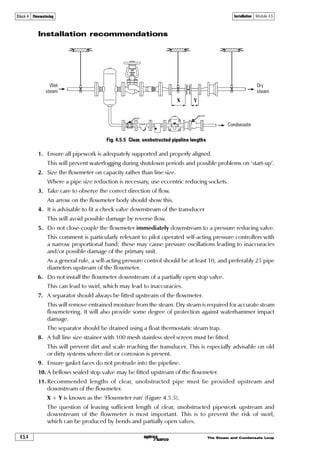
68. The Steam and Condensate Loop4.4.14
Instrumentation Module 4.4Block 4 Flowmetering
Example 4.4.6
Consider a steam flowmeter fitted with pressure reading equipment, but not temperature reading
equipment. The flowmeter thinks it is reading saturated steam at its corresponding temperature.
With superheated steam at 4 bar g and 10°C superheat passing through the flowmeter, determine
the actual flowrate if the flowmeter displays a flowrate of 250 kg/h.
Equation 4.4.5 can be used to calculate the actual value from the displayed value.
[ ]
!$
6p‡ˆhyÉhyˆr Ã2Ã! 'Ãxt u
ÃÃ #$
=
With steam at a line pressure of 4 bar g and 10°C superheat, the displayed value of mass flow will
be 14.5% higher than the actual value.
For example, if the display shows 250 kg/h under the above conditions, then the actual flowrate
is given by:
Equation 4.4.5
9v†ƒyh’rqÉhyˆr6p‡ˆhyÉhyˆr ÈÃr……‚…
=
⎡ ⎤⎛ ⎞
⎜ ⎟⎢ ⎥⎝ ⎠⎣ ⎦

69. The Steam and Condensate Loop 4.4.15
Block 4 Flowmetering Instrumentation Module 4.4
Answers 1:b,2:d,3:a,4:b,5:c,6:b
Questions
1. A flowmeter used on superheated steam at 10 bar g and 234°C displays a flow of
1 000 kg/h. If the flowmeter does not incorporate temperature and pressure
compensation what is the actual flowrate?
a| 1 000 kg/h ¨
b| 571 kg/h ¨
c| 1 339 kg/h ¨
d| 822 kg/h ¨
2. A flowmeter measuring differential pressure calibrated for saturated steam at 7 bar g
displays a flowrate of 800 kg/h. What will be the effect of the steam being 3% wet?
a| The actual flow will remain the same as that indicated ¨
b| The actual flow will be 406 kg/h ¨
c| The actual flow will be 788 kg/h ¨
d| The actual flow will be 812 kg/h ¨
3. A typical DP cell used with a measuring differential pressure flowmeter……
a| Senses the pressure either side of the flowmetering device and relays a corresponding
electrical signal to a display processor ¨
b| Compares the pressure downstream of the flowmetering device with a fixed upstream
pressure and volume, and relays the difference by means of a corresponding
electrical signal to a display processor ¨
c| Senses differential pressure across the flowmetering device, and density of the steam
at the designed upstream pressure and passes this information to a display processor ¨
d| Senses changes in pressure upstream of the flowmetering device and relays a
corresponding electrical signal to a display processor ¨
4. An orifice plate flowmeter is designed for use on saturated steam at 5 bar g
but for much of its life it operates on steam at 4 bar g and displays a flowrate
of 1 200 kg/h. Will the display at 4 bar g be accurate if the flowmeter is not fitted
with density compensation?
a| No, the actual flowrate will be 1 316 kg/h ¨
b| No, the actual flowrate will be 1 100 kg/h ¨
c| Yes ¨
d| No, the flowmeter will be outside its turndown ratio ¨
5. The steam in question 4 is thought to be very wet. What effect will this have?
a| The orifice will erode resulting in the actual flow being less than that indicated ¨
b| The effect will be insignificant ¨
c| The actual flowrate will be higher than the indicated flowrate ¨
d| The actual flowrate will be less than the indicated flowrate ¨
6. A flowmeter measuring differential pressure is installed on a system where the
pressure can vary between 20 bar g and 1 bar g. Which of the following could
cause inaccuracy of the flowmeter?
a| The steam becoming superheated because of the pressure drop ¨
b| Density compensation not being incorporated ¨
c| The high pressure turndown ¨
d| All of the above ¨

70. The Steam and Condensate Loop4.4.16
Instrumentation Module 4.4Block 4 Flowmetering

71. The Steam and Condensate Loop 4.5.1
Block 4 Flowmetering Installation Module 4.5
Module 4.5
Installation
SC-GCM-47CMIssue1©Copyright2005Spirax-SarcoLimited

72. The Steam and Condensate Loop4.5.2
Installation Module 4.5Block 4 Flowmetering
Installation
The manufacturer should always supply installation data with the product as this will lay
down specific requirements such as the minimum lengths of unobstructed pipe to be provided
upstream and downstream of the flowmeter. It is usual for the flowmeter supplier to be able
to offer advice and relay recommendations regarding the installation requirements of his
particular flowmeter.
Statistics show that over a third of flowmeter problems are due to poor installation. No steam
flowmeter, however good its design and thorough its manufacture, can cope if little attention is
paid to its installation and the layout of the steam system.
Steam quality
Dry steam
Steam should always be provided in as dry a condition as possible at the point of metering.
Module 4.4 has already demonstrated that wet steam will cause inaccuracies and can physically
damage some types of flowmeter.
Fig. 4.5.1 Typical separator
Wet
steam
in
Air and
condensable gases
vented
Dry
steam
out
Moisture to trapset
A simple but effective method of drying
wet steam is to install a separator upstream
of the flowmeter. Entrained moisture
impinges on the baffle plates and the
heavy droplets fall to the bottom and are
drained away via a properly sized and
selected steam trap set. Independent tests
show that it is possible to achieve a 99%
dryness fraction over a wide range of flows
by use of a high efficiency separator as
shown in Figure 4.5.1.
The separator has one other important
benefit: Slugs of water impacting on any
steam flowmeter (i.e. waterhammer) can
cause severe mechanical damage. Fitting
a separator before a steam flowmeter will
reduce the resulting impact pressure from
water slugs by up to 90%, affording
considerable protection to any expensive
flowmetering device.
The separator with its drain trap ensures
efficient condensate removal ahead of the
flowmeter. But any low points where the
steam main rises to a higher level should
also have drain trap points that are
adequately sized and correctly selected.
It is also worthwhile ensuring that air
and other entrained gases are removed by
fitting an air vent in the steam line.
The separator shown in Figure 4.5.1 has a
top connection suitable for an automatic
air vent that will help to remove
incondensable gases prior to the
flowmetering station. Figure 4.5.2 illustrates
a combined drain trap point and venting
station at the end of a steam main.

73. The Steam and Condensate Loop 4.5.3
Block 4 Flowmetering Installation Module 4.5
Fig. 4.5.2 Condensate and air removal at the end of a steam main
Clean steam
A pipeline strainer (Figure 4.5.3)
should be fitted ahead of the
flowmeter. This will remove any larger
pieces of scale, swarf or other pipeline
debris, which would otherwise
damage the primary device. The
internal strainer device should be
cleaned periodically, particularly
during the initial start-up of a new
installation.
As with any steam pipeline strainer,
the strainer should be installed with
the body horizontal to avoid creating
an accumulation of condensate and
hence a reduction in the screening
area (Figure 4.5.4). Fig. 4.5.3 Cut section of a typical pipeline strainer
Steam out via branch line
Steam flow
Air vent
Trap set
Steam
in
Steam
out
100 mesh
screen
Condensate Drain pocket
➧
➧
Maintenance
The provision of valves either side of the flowmeter should be considered for isolation purposes,
since inspection, maintenance and perhaps even ‘removal for calibration’ will sometimes be
necessary. Such valves should be of the fully open or fully closed type, which present the least
resistance to flow, such as full bore ball valves. In addition, a valved bypass, or a make-up piece
to act as a temporary replacement if the flowmeter is removed from the pipeline, will solve the
problem of interrupting the steam supply during maintenance procedures. Both pipework and
flowmeter must be adequately supported and properly aligned with a slight fall to the last drain
point ahead of the flowmeter. Pipework should also be properly and effectively insulated to
minimise radiation losses and further condensation.
Fig. 4.5.4 Correct strainer orientation for steam or gas applications

74. The Steam and Condensate Loop4.5.4
Installation Module 4.5Block 4 Flowmetering
Installation recommendations
Fig. 4.5.5 Clear, unobstructed pipeline lengths
1. Ensure all pipework is adequately supported and properly aligned.
This will prevent waterlogging during shutdown periods and possible problems on ‘start-up’.
2. Size the flowmeter on capacity rather than line size.
Where a pipe size reduction is necessary, use eccentric reducing sockets.
3. Take care to observe the correct direction of flow.
An arrow on the flowmeter body should show this.
4. It is advisable to fit a check valve downstream of the transducer
This will avoid possible damage by reverse flow.
5. Do not close-couple the flowmeter immediately downstream to a pressure reducing valve.
This comment is particularly relevant to pilot operated self-acting pressure controllers with
a narrow proportional band; these may cause pressure oscillations leading to inaccuracies
and/or possible damage of the primary unit.
As a general rule, a self-acting pressure control should be at least 10, and preferably 25 pipe
diameters upstream of the flowmeter.
6. Do not install the flowmeter downstream of a partially open stop valve.
This can lead to swirl, which may lead to inaccuracies.
7. A separator should always be fitted upstream of the flowmeter.
This will remove entrained moisture from the steam. Dry steam is required for accurate steam
flowmetering. It will also provide some degree of protection against waterhammer impact
damage.
The separator should be drained using a float thermostatic steam trap.
8. A full line size strainer with 100 mesh stainless steel screen must be fitted.
This will prevent dirt and scale reaching the transducer. This is especially advisable on old
or dirty systems where dirt or corrosion is present.
9. Ensure gasket faces do not protrude into the pipeline.
10. A bellows sealed stop valve may be fitted upstream of the flowmeter.
11. Recommended lengths of clear, unobstructed pipe must be provided upstream and
downstream of the flowmeter.
X + Y is known as the ‘Flowmeter run’ (Figure 4.5.5).
The question of leaving sufficient length of clear, unobstructed pipework upstream and
downstream of the flowmeter is most important. This is to prevent the risk of swirl,
which can be produced by bends and partially open valves.
Wet
steam
Dry
steam
Condensate
X Y

75. The Steam and Condensate Loop 4.5.5
Block 4 Flowmetering Installation Module 4.5
Fig. 4.5.6 Flow straighteners
Correct sizing of the flowmeter is also essential and most manufacturers will recommend maximum
and minimum flowrates for each size of flowmeter.
If the flowmeter to be used is smaller than the pipeline into which it is to be fitted, reductions in
pipe size should be achieved by using eccentric reducers (Figure 4.5.7). This will prevent the
collection of condensate at a lowpoint - as would be the result if concentric reducers were
used. The reduction in pipe size should be achieved at the nearest point to the flowmeter consistent
with maintaining the required flowmeter run.
Rotation
Forward motion
Types of ‘flow straighteners’
Fig. 4.5.7 Pipe size reduction
✓
✗Flow
Concentric reducer
Steam flowmeter
Eccentric reducer
Flowmeter run
Steam flowmeter
Flow
Some types of flowmeter are more susceptible to swirl than others. Some manufacturers
recommend the use of flow straighteners to remove swirl (Figure 4.5.6). However, it is preferable
to do all that is possible to prevent the risk of swirl by providing an adequate flowmeter run since
flow straighteners in steam systems can entrain surface water. It may even be preferable to select
a steam flowmeter that is less susceptible to the effects of swirl.
Low point allowing collection of condensate

76. The Steam and Condensate Loop4.5.6
Installation Module 4.5Block 4 Flowmetering
System design considerations
Adopting a structured approach to steam flowmetering will help to ensure that:
o The design objectives are achieved.
o No elements of the design are omitted.
o The benefits are maximised.
o The financial outlay is minimised.
There are two main elements to such an approach:
1. Consideration of the existing steam supply system
The planner should identify any future changes to the plant or process that may affect the installation
of steam flowmeters, and should consider whether the installation of flowmeters is likely to act as
a catalyst for such changes. Alterations to the system, for example, may involve blanking off
redundant sections of steam mains, rerouting pipework, or generally improving the condition of
pipe layout and/or insulation.
2. Identifying the aim of installing steam flowmetering
Typically, one or more of the following design criteria will be clearly defined:
o To provide information for accounting purposes, such as departmental allocation of costs.
o To facilitate custody transfer, for example where a central station sells steam to a range of clients.
o To facilitate Monitoring and Targeting (M and T) policies and observe trends.
o To determine and monitor energy utilisation and efficiency.
Each of the above criteria imposes different limitations on the design of the steam flowmetering
system.
If flowmetering is to be used for accounting purposes or for custody transfer, it will be necessary
to install a sufficient number of flowmeters for consumption to be assigned to each of the cost
centres. Also, if the product being sold is energy not steam, flowmeters will also have to be
installed on the condensate return lines, as this hot water will have a heat value. For both
applications, the highest possible standard of flowmetering will be required, particularly with
respect to accuracy, turndown ratio, and repeatability.
The system may also require check flowmetering so that consumption can be proven correct. It
should be noted that confidence in any monitoring system, once lost, is very difficult to restore.
A system should also include measurement of the system losses incurred as a result of supplying
steam to a particular location. This implies that flowmeter positions should be located as near to
the boiler house as possible.
In M and T applications and in the determining of energy efficiency, the important flowmetering
criterion is repeatability. The user will be more interested in trends in consumption rather than
absolute values.
Determining flowmeter arrangements
Once the system layout has been determined, and the data required to accurately measure the
energy consumption of the system / plant has been decided, the number and location of required
flowmeters can be contemplated. This requires consideration of the site as a whole including
the steam main from the boiler house.
Figure 4.5.8 shows four possible layouts for the same system.