DIFFUSER ANGLE CONTROL TO AVOID FLOW SEPARATION

International Journal of Technical Research and Applications e-ISSN: 2320-8163,
www.ijtra.com Volume 2, Issue 5 (Sep-Oct 2014), PP. 16-21
16 | P a g e
DIFFUSER ANGLE CONTROL TO AVOID FLOW
SEPARATION
Vinod Chandavari1
, Mr. Sanjeev Palekar2
M.Tech (APT), Department of Aerospace Propulsion Technology
Visvesvaraya Technological University - CPGS
Bangalore, Karnataka, India
1
vinodchandavari@gmail.com, 2
aero.sanjeev@gmail.com
Abstract— Diffusers are extensively used in centrifugal
compressors, axial flow compressors, ram jets, combustion
chambers, inlet portions of jet engines and etc. A small change in
pressure recovery can increases the efficiency significantly.
Therefore diffusers are absolutely essential for good turbo
machinery performance. The geometric limitations in aircraft
applications where the diffusers need to be specially designed so
as to achieve maximum pressure recovery and avoiding flow
separation.
The study behind the investigation of flow separation in a planar
diffuser by varying the diffuser taper angle for axisymmetric
expansion. Numerical solution of 2D axisymmetric diffuser model
is validated for skin friction coefficient and pressure coefficient
along upper and bottom wall surfaces with the experimental
results of planar diffuser predicted by Vance Dippold and
Nicholas J. Georgiadis in NASA research center [2]
.
Further the diffuser taper angle is varied for other different
angles and results shows the effect of flow separation were it is
reduces i.e., for what angle and at which angle it is just avoided.
Keywords: Planar Diffuser, CFD, Taper angle, Flow Separation.
I. INTRODUCTION
Diffusers are integral parts of jet engines and many other
devices that depend on fluid flow. Performance of a
propulsion system as a whole is dependent on the efficiency of
diffusers. Identification of separation within diffusers is
important because separation increases drag and causes inflow
distortion to engine fans and compressors. Diffuser flow
computations are a particularly challenging task for
Computation Fluid Dynamics (CFD) simulations due to
adverse pressure gradients created by the decelerating flow,
frequently resulting in separation.
These separations are highly dependent on local turbulence
level, viscous wall effects, and diffuser pressure ratio, which
are functions of the velocity gradients and the physical
geometry. The diffuser is before the combustion chamber that
ensures that combustion flame sustenance and velocities are
small [2]
.
1.1 What is the meaning of Separation or Reverse Flow?
The designing of an efficient combustion system is easier
if the velocity of the air entering the combustion chamber is as
low as possible. The natural movement of the air in a diffusion
process is to break away from the walls of the diverging
passage, reverse its direction and flow back in the direction of
the pressure gradient, as shown in figure 1.1 air deceleration
causes loss by reducing the maximum pressure rise [4]
.
Fig: 1.1 Diffusing Flow
Buice, C.U. and Eaton, J.K [1]
, was carried out the
Experimental work using a larger aspect ratio experimental
apparatus, paying extra attention to the treatment of the
endwall boundary layers. They are titled as “Experimental
Investigation of Flow through an Asymmetric Plane Diffuser,”
The results of this experiment are compared to the results of
different calculations made for the same diffuser geometry and
Reynold number. One of the calculation is Large Eddy
Simulation (LES). The other is a Reynold Averaged Navier
Stokes (RANS) calculation using v2
-f turbulence model. Both
calculations captured the major features of the flow including
separation and reattachment.
Vance Dippold and Nicholas J. Georgiadis[2]
, they have been
performed “Computational Study of Separating Flow in a
Planar Subsonic Diffuser” in National Aeronautics and Space
Administration is computed with the SST, k-ε, Spalart-
Allmaras and Explicit Algebraic Reynolds Stress turbulence
models are compared with experimentally measured velocity
profiles and skin friction along the upper and lower walls.
Olle Tornblom[3]
, repeated the experimental work of Buice,
C.U. and Eaton, J.K, “Experimental study of the turbulent
flow in a plane asymmetric diffuser”, the flow case has been
concentrated on in an uniquely composed wind-tunnel under
overall controlled conditions. A similar study is made where
the measured turbulence data are utilized to assess an explicit
algebraic Reynolds stress turbulence model (EARSM) and
coefficient of pressure is measured.
In this study diffuser gives an idea of choosing the turbulence
model and to avoid separation flow by varying the taper angle
(7º, 8º, 9º and 10º).
The diffuser model and Fluent 14.5 are used, to study the
diffuser characteristics with the effect of various factors like
Pressure coefficient and Skin friction coefficient. Obtained
results are validated against the known experimental results
carried out by Vance Dippold and Nicholas J. Georgiadis [2]
.
II. PHYSICAL MODEL AND MESH
Diffuser geometric configuration with the height of the inlet
channel H = 0.015 meters and the diffuser has a 10ᴼ expansion
taper angle and is 21H in length. At the end of the expansion,
the diffuser channel is 4.7H in height. Figure 2.1 shows the
schematic diagram of diffuser [1]
.

17 | P a g e
Fig: 2.1 Shows the schematic diagram of Diffuser
Figure 2.2 shows the computational domain of 2D that mimics
the physical model. The diffuser apparatus can be divided into
three sections: an inflow channel, the asymmetric diffuser, and
an outflow channel. Figure 2.3 shows the 2D structured mesh
for computational domain. Mesh having 41511 nodes and
41000 elements.
Mesh Quality:
Orthogonal Quality is ranges from 0 to 1, where values close
to 0 correspond to low quality. Hence the
 Minimum Orthogonal Quality = 0.945334629648056
 Y plus value= 1.03
Fig: 2.2 Computational domain
Fig: 2.3 Computational Domain with Mesh
III. NUMERICAL PROCEDURE
This project implemented steady Reynolds Averaged Navier-
Stokes equations (RANS) in the ANSYS FLUENT flow
simulation program. For all cases, a two-dimensional, double-
precision flow solver was used. It was assumed that the
application of steady RANS equations was sufficient for this
study because the flow through the diffuser user is steady in
the mean. In this study, SST-K-ω turbulence models were used
with varying complexities and formulations. Understandably,
the increased complexity (i.e., increased number of equations)
requires more computational time. Thus, the selection of
turbulence models with varying complexities provides the
opportunity to observe a correlation between modeling
accuracy and computational time [4]
.
Identical boundary conditions were used for all turbulence
models. In particular, the inlet conditions were specified as a
constant velocity profile corresponding to the bulk inlet
velocity, Ub = 20 m/s.
All turbulence models implemented a COUPLED scheme to
couple the pressure and velocity. Furthermore, the spatial
discretization was accomplished by a second-order accurate
upwind scheme for the momentum and a FLUENT standard
scheme for the pressure. Any additional closure equations for
the various turbulence models were spatially discretized by
second-order accurate upwind schemes. In all cases, the
corresponding calculation residuals were monitored to
convergence at 1*10-05
. These residuals included continuity, x-
velocity, and y-velocity for all turbulence models. Beyond
these generic residuals, any additional closure equations gave
additional terms to monitor. The fluid properties were
carefully chosen to ensure a matched Reynolds number with
the experimental data. Specifically, the fluid density was
chosen to be 1.225 kg/m3 and the dynamic viscosity was
selected to be 1.789*10-05
kg/m-s. The combination of these
values yields the appropriate Reynolds number based on inlet
channel height, ReH = 20,000.
IV. VALIDATION
The suitability of solver selection, turbulence model,
numerical scheme, discretisation method and convergence
criteria used in the present study is validated by comparing the
skin friction coefficient and pressure coefficient along the X/H
with the experimental data of Vance Dippold and Nicholas J.
Georgiadis[2]
. Among various turbulence models available in
the fluent code, SST-k-ω model are tested with different taper
angle (7º, 8º, 9º and 10º).
The figures 4.1.1 and 4.1.3 shows skin friction coefficient is
0.006 of Bottom_wall and Top_wall respectively, figure 4.2.1
shows the Pressure coefficient and the figure 4.1.2, 4.1.4 and
4.2.2 shows computational results obtained are in better
agreement with the known experimental results as follows.
Table: 4.2 Comparison of Experimental Results with Computational
Results
Parameters Experimental Computational
Taper Angle 10 º 7 º 8 º 9 º 10 º
Pressure
coefficient
0.73 to 0.85 0.882 0.880 0.873 0.85
Skin friction
coefficient
0.006 to 0.0063 0.0064 0.0065 0.0066 0.006
Velocity
(m/s)
Min -1.156 0 -0.146 -0.723 -1.156
Max 22.845 22.845 22.845 22.845 22.845

18 | P a g e
Table 4.2 demonstrates the correlation distinctive parameters
of experimental results with computational results. This table
demonstrates the how the taper angle decreases pressure
coefficient expands and skin friction coefficient diminishes
this implies the flow separation is bit by bit diminishes.
Fig: 4.1.1 Experimental results of Bottom_wall skin friction along with
the X/H using the SST model at 10ᴼ taper angle [2]
Fig: 4.1.2 Comparison of Computational Results with Experimental
Results of Bottom_wall skin friction along with the X/H using the SST
model at 10ᴼ taper angle
Fig: 4.1.3 Experimental results of Top_wall skin friction along with the
X/H using the SST model at 10ᴼ taper angle [2]
Fig: 4.1.4 Comparison of Computational Results with Experimental
Results of Top_wall skin friction along with the X/H using the SST model
at 10ᴼ taper angle
Fig: 4.2.1 Experimental results of pressure coefficient (Cp) at 10ᴼ taper
angle along with the X/H
Fig: 4.2.2 Computational Results of Pressure Coefficient, bottom and Top
wall at 10ᴼ taper angle
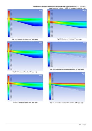
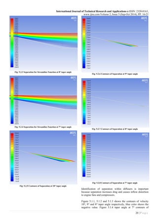
V. RESULTS AND DISCUSSION
The results are obtained from the CFD by applying the
experimental condition to the computational model with
variation of taper angle 7ᴼ, 8ᴼ, 9ᴼ, and 10ᴼ, were measured for
different contours plots, figure 5.1.1, 5.1.2, 5.1.3, and 5.1.4
shows the contours of velocity, figure 5.2.1, 5.2.2, 5.2.3, and
5.2.4 shows the separation for streamline functions and figure
5.2.5, 5.2.6, 5.2.7, and 5.2.8 shows contours of separation
flow.

19 | P a g e
Fig: 5.1.1 Contours of Velocity at 10ᴼ taper angle
Fig: 5.2.1 Separation for Streamline Function at 10ᴼ taper angle

20 | P a g e
Fig: 5.2.5 Contours of Separation at 10ᴼ taper angle
Identification of separation within diffusers is important
because separation increases drag and causes inflow distortion
to engine fans and compressors.
Figure 5.1.1, 5.1.2 and 5.1.3 shows the contours of velocity
10ᴼ, 9ᴼ and 8ᴼ taper angle respectively, blue color shows the
negative value. Figure 5.1.4 taper angle at 7ᴼ contours of

21 | P a g e
velocity doesn’t shows negative value it means that the
separation flow is avoided at 7ᴼ taper angle.
VI. CONCLUSION
From the present study it is evident that when the taper angle
is decreased, the skin friction coefficient drops & pressure
coefficient rises, as result the flow separation follows a
diminishing trend
The optimum taper angle is 7ᴼ below which there is no flow
separation at all but going beyond it gives rise to flow
separation
VII. SCOPE FOR FUTURE WORK
The proposed next work for the present configuration is,
simulating for 3D structured mesh configuration to these taper
angle varieties and as in the present work the contrast in 2D
taper angle we can figure it for variety taper angle, and 3D
configuration simulation is possible for the impact of
expectation taper angle.
REFERENCES
[1] Buice, C.U. and Eaton, J.K., “Experimental Investigation of
Flow Through an Asymmetric Plane Diffuser,” 1997
[2] Vance Dippold and Nicholas J. Georgiadis., “Computational
Study of Separating Flow in a Planar Subsonic Diffuser,”
NASA, October 2005
[3] Olle Tornblom., “Experimental study of the turbulent flow in a
plane asymmetric diffuser,” 2003
[4] Reid A. Berdanier., “Turbulent flow through an asymmetric
plane diffuser”, Purdue University, April-2011
[5] Arthur H Lefebvre and Dilip R. Ballal., “Gas Turbine
Combustion-Alternative Fuels and Emissions”, CRC Press
Taylor & Francis Group, Third Edition pp.79 – 112 – 2010
[6] Gianluca Iaccarino., “Predictions of a Turbulent Separated Flow
Using Commercial CFD Codes,” 2001
[7] Obi, S., Aoki, K., and Masuda, S., “Experimental and
Computational Study of Turbulent Separating Flow in an
Asymmetric Plane Diffuser,” Ninth Symposium on Turbulent
Shear Flows, Kyoto, Japan, August-1993.
[8] Dheeraj Sagar, Akshoy Ranjan Paul Et al., “Computational
fluid dynamics investigation of turbulent separated flows in
axisymmetric diffusers,” 2011
[9] E.M. Sparrow and J.P. Abraham., Et al. “Flow separation in a
diverging conical duct: Effect of Reynolds number and
Divergence angle,” 2009.

DIFFUSER ANGLE CONTROL TO AVOID FLOW SEPARATION

More Related Content

What's hot

Viewers also liked

Similar to DIFFUSER ANGLE CONTROL TO AVOID FLOW SEPARATION

More from International Journal of Technical Research & Application

Recently uploaded

DIFFUSER ANGLE CONTROL TO AVOID FLOW SEPARATION