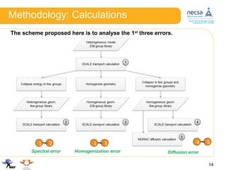
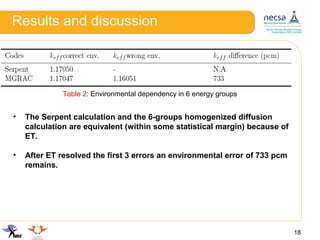
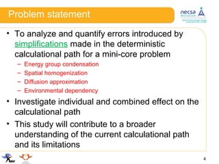
This document discusses modelling errors introduced in the deterministic calculational path for analyzing a mini-core reactor problem. It presents the methodology used to quantify individual and combined effects of simplifications like energy group condensation, spatial homogenization, and the diffusion approximation. The results show that spectral, diffusion, and environmental errors are significant for a 6-group model of the mini-core problem, with combined errors over 4000 pcm. Equivalence theory resolved errors except for a remaining 733 pcm environmental error. Future work will further investigate environmental errors and apply these findings to improve reactor modelling calculations.

1. Analysis and quantification
of modelling errors
introduced in the
deterministic calculational
path applied to a mini-core
problem
SAIP 2015 conference
01 July 2015
Speaker: Mr. T.P. Gina(1), (2)
Supervisors: Prof. S.H. Connell(1)
Mrs. S.A.
Groenewald(2)
Dr. W.R.
Joubert (2)
Affiliation: UJ(1)
, Necsa(2)

2. Outline
1. Introduction
2. Problem statement
3. Neutronics modelling
4. Methodology
5. Results and discussions
6. Conclusion
2

3. Introduction
• What is reactor modelling?
– Set of algorithms & computer codes to perform reactor
calculations
– Understand and predict core behaviour
• Why is reactor modelling error analysis
important?
• Part of a bigger study focused on improving the
errors made in modelling MTRs.
– Modelling error analysis is done on a mini-core problem
– The approach defined will be applied to a full-core MTR model
3

4. Problem statement
• To analyze and quantify errors introduced by
simplifications made in the deterministic
calculational path for a mini-core problem
– Energy group condensation
– Spatial homogenization
– Diffusion approximation
– Environmental dependency
• Investigate individual and combined effect on the
calculational path
• This study will contribute to a broader
understanding of the current calculational path
and its limitations
4

5. Neutronics modelling
• Determines neutron flux distribution
• It describes the motion and interaction of
neutrons with nuclei in the reactor core.
– 7 independent variables [x, y, z, θ, ϕ, E, t]
– Flux is the dependent variable.
5
(Duderstadt and Hamilton 1976)

6. Neutronics modelling...
• For day-to-day reactor calculations, the
deterministic approach is used to solve transport
equation because of its calculational efficiency
• This approach involves discretizing variables of
the transport equation to set of equations.
• The transport equation is solved numerically
• The deterministic method is applied to reactor
analysis calculations via a two-step process.
6

7. Neutronics modelling...
7
Here is a two-step deterministic
calculational path.
1.Perform a detailed 2D transport
calculation on each assembly type.
– Use solution to simplify geometry
and energy representation
– Produce spatially homogenized,
energy condensed assembly
cross section for each reactor
component.
2.Use nodal cross sections in the
diffusion calculation to simulate full
core.

8. Neutronics modelling...
8
Homogenization and energy
condensation
The simplifications made in geometry and
energy representation in the node involve
performing a fine energy group
heterogeneous transport calculation.
Heterogeneous flux is used as weighting
function to homogenise and collapse cross-
sections to fewer (10s) energy groups
Each node has a constant set of few-
groups homogenized nodal parameters that
preserve the transport solution in an average
sense.
1.E+00
1.E+01
1.E+02
1.E+03
1.E+04
1.E+05
1.E-05 1.E-03 1.E-01 1.E+01 1.E+03 1.E+05 1.E+07
Crosssection(barn)
Energy (eV)
Total cross section for U235
in 238 and 6 energy groups
U235 total in 238 groups
U235 total in 6 groups

9. Neutronics modelling...
9
Reaction rates preserved
(Smith 1980)

10. Neutronics modelling…
• Diffusion approximation
– The diffusion equation is derived from transport
equation
10
Fick’s Law
(Duderstadt and Hamilton 1976)
Diffusion approx. theory is valid:
•Slowly varying current density in time
•Isotropic scattering
•Angular flux distribution is linearly
anisotropic
Diffusion approx. theory is invalid:
•In strongly absorbing media
•Near the boundary where material
properties change dramatically over mfp
type distances
•Near localized sources

11. Neutronics modelling…
• Environmental dependency
– Due to the transport solution’s approximate boundary conditions
– Cross-sections are generated in an environment that is not exact
to the environment where they’ll be used in the core calculation.
– Using cross sections from an infinite environment for the fuel
elements in a different core environment an environmental error
is introduced in the model.
• The first 3 errors are typically addressed by
using the equivalence theory (ET).
• ET reproduces node-integrated parameters of
the known heterogeneous solution (Smith K.S).
11

12. Methodology
• We want to numerically quantify the errors made
in a mini-core problem.
• With reflective boundary conditions
12
Fuel-Water model

13. Methodology: Codes
• Code systems used:
– SCALE6.1 (NEWT)
• 2D transport solver
• Uses Sn (Discrete Ordinate Method)
– OSCAR-4 (MGRAC)
• 3D diffusion solver
• Uses the Multi-group Analytic Nodal Diffusion Method
– Serpent
• Uses the Monte Carlo stochastic method
• 3D and continuous energy
13

14. Methodology: Calculations
1 2 1 3 4 5
14
Spectral error Homogenization error Diffusion error
The scheme proposed here is to analyse the 1st
three errors.

15. Methodology: Calculations
15
•The Serpent code was used to generate correct
and approximated fuel cross sections.
•Functionality exists to generate nodal equivalence
parameters from Serpent calculations.
•Two MGRAC calculations were set up
– One with no environmental error and one with
environmental error
•Compare k-effs.
The scheme proposed here is to analyse environmental error.

16. Results and discussion
• The k-eff is measure of criticality
• Error in k-eff is measured in pcm as:
• Error in k-eff > 500pcm is considered large.
• Reference k-eff = 1.17073
16

17. Results and discussion
17
2-groups 4-groups 6-groups
Combined error (pcm) -3472 -4406 -4113
Table 1: Errors from the first 3 simplifications

18. Results and discussion
18
Table 2: Environmental dependency in 6 energy groups
• The Serpent calculation and the 6-groups homogenized diffusion
calculation are equivalent (within some statistical margin) because of
ET.
• After ET resolved the first 3 errors an environmental error of 733 pcm
remains.

19. Results and discussion
• Spectral error and reactivity increase with the
decrease in number of groups
• Homogenization error is small
• Diffusion error is up to 6000 pcm larger in 2-
groups
• All 3 simplifications reduce calculational time.
19

20. Conclusion
20
• All simplification to the deterministic calculational
path were investigated for a mini-core problem.
• Spectral, diffusion and environmental error were
significant for a mini-core problem in 6-groups.
• ET was successfully used to resolve all errors
except environmental.
• Future work
– Environmental error will be investigated further.
– More models will be investigated.
– Results will be used in an on-going research project
to improve current calculational path.

21. THANK YOU
21