Download as PPS, PPTX
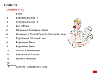
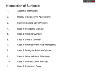
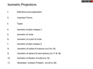


This document provides an overview of topics related to engineering graphics and geometric constructions including: 1. Engineering curves such as involutes, cycloids, trochoids, spirals, and helices. 2. Loci of points including definitions, basic locus cases, and problems involving oscillating and rotating links. 3. Orthographic projections including basics, types of drawings and views, planes of projection, and methods. 4. Converting pictorial views to orthographic views using first and third angle methods with illustrations. 5. Projecting points, lines, planes, and solids including their definitions, notations, procedures, examples, and problem sets. 6. Sections


![Typicalproblem(thedirectdata[1].com)](https://cdn.slidesharecdn.com/ss_thumbnails/typicalproblemthedirectdata1-170802182647-thumbnail.jpg?width=640&height=640&fit=bounds)
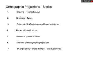
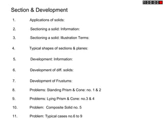
![Sectionanddevelopment(thedirectdata[1].com)](https://cdn.slidesharecdn.com/ss_thumbnails/sectionanddevelopmentthedirectdata1-170802182625-thumbnail.jpg?width=640&height=640&fit=bounds)

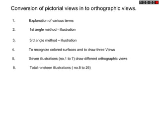
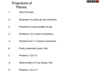
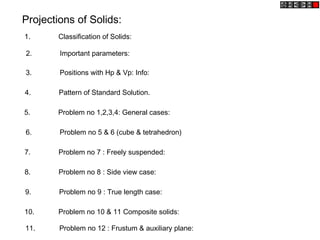
![Projectionofsolids(thedirectdata[1].com)](https://cdn.slidesharecdn.com/ss_thumbnails/projectionofsolidsthedirectdata1-170802182501-thumbnail.jpg?width=640&height=640&fit=bounds)
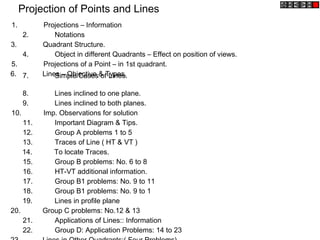
![Projectionoflines(thedirectdata[1].com)](https://cdn.slidesharecdn.com/ss_thumbnails/projectionoflinesthedirectdata1-170802182419-thumbnail.jpg?width=640&height=640&fit=bounds)
![Ortographicprojection(thedirectdata[1].com)](https://cdn.slidesharecdn.com/ss_thumbnails/ortographicprojectionthedirectdata1-170802182401-thumbnail.jpg?width=640&height=640&fit=bounds)
![Lociofpoint(thedirectdata[1].com)](https://cdn.slidesharecdn.com/ss_thumbnails/lociofpointthedirectdata1-170802182346-thumbnail.jpg?width=640&height=640&fit=bounds)
![Excerciseeg(thedirectdata[1].com)](https://cdn.slidesharecdn.com/ss_thumbnails/excerciseegthedirectdata1-170802182329-thumbnail.jpg?width=640&height=640&fit=bounds)
![Ellipsebygenmethod(thedirectdata[1].com)](https://cdn.slidesharecdn.com/ss_thumbnails/ellipsebygenmethodthedirectdata1-170802182324-thumbnail.jpg?width=640&height=640&fit=bounds)

![Curves1(thedirectdata[1].com)](https://cdn.slidesharecdn.com/ss_thumbnails/curves1thedirectdata1-170802181913-thumbnail.jpg?width=640&height=640&fit=bounds)


