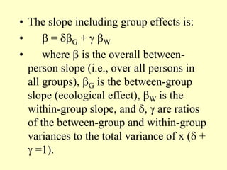
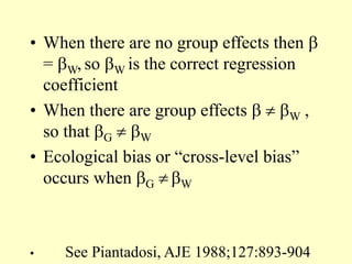
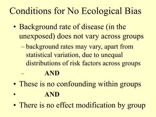
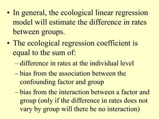
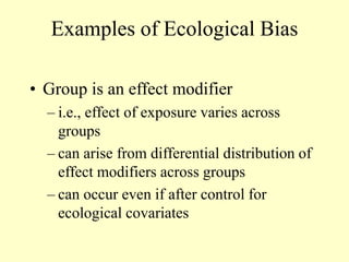
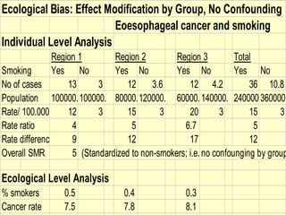
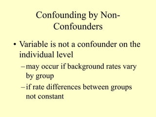
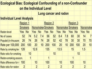
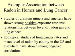
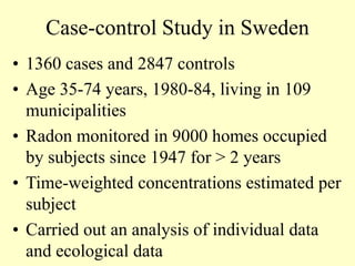
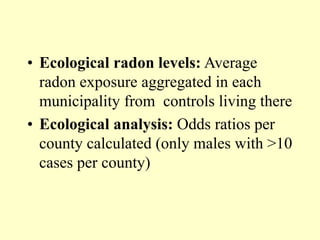
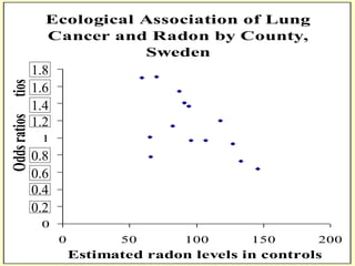
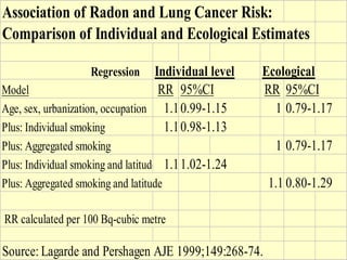
This document discusses ecological studies, which investigate the distribution of health outcomes and their determinants between groups rather than individuals. While individual-level data may not be available, ecological studies can still provide useful information. However, inferences made from ecological data to individuals may be biased due to factors varying between groups like background rates, confounding, or effect modification. Conditions where ecological bias does not occur include no variation in background rates or effects between groups. Solutions proposed to address ecological bias include obtaining more detailed covariate data or conducting individual-level studies. The document provides examples of potential biases and compares individual versus ecological estimates using a study of radon exposure and lung cancer risk.

1. An Introductory Lecture to
Environmental Epidemiology
Part 5. Ecological Studies.
Mark S. Goldberg
INRS-Institut Armand-Frappier,
University of Quebec, and
McGill University
July 2000

2. Ecological Studies
• Definition: An investigation of the
distribution of health and its
determinants between groups of
individuals.
• The degree to which studies are purely
ecological can vary considerably.

3. Reasons for Ecological Studies
• Data on the individual level not available
• Individual exposure measurements not
available, but grouped level data are (e.g.,
mean radon gas levels from county-wide
surveys)
• Comparison between large jurisdictional units
(e.g., comparison of breast cancer rates with
mean daily fat intake between countries)

4. • Easy, quick, and inexpensive
• Design limitations (e.g., Harvard Six-
cities study; see Part 1)
• Interest in ecological effects (e.g., does
increasing taxes on tobacco reduce
consumption in different jurisdictions?)

5. Measurement variables
• Aggregated measures: summaries of
attributes calculated from data on
individuals for whole populations in
well-defined geographic regions
• Examples: mean income;
percentage of families below the
poverty line; mean number of
household members

6. • Group level measures: estimates of
(environmental) attributes that have
individual analogues. Usually obtained
from surveys.
• Examples: maximum daily
exposure to ozone; mean annual
exposures to radon gas; daily mean
levels of environmental tobacco smoke
in public buildings

7. • Global measures (contextual):
attributes that pertain to groups and do
not have analogues at the individual
level
• Examples: total area of green space;
number of private medical clinics;
population density

8. Types of studies
• Individual level: Well defined target and
study populations and data available on
individuals for all (or most) covariates.
• Example: Cross-sectional study of
respiratory symptoms and exposure to
environmental tobacco smoke among
children living in Mexico City.

9. • Purely ecologic: No data on
individuals
• Example: Average per capita
consumption of snuff and age-sex-race
standardized mortality rates of oral
cancer. Comparisons at the county
level.

10. • Partially ecologic: Some individual data
available.
• Example: A study of low birth weight and
environmental exposures to biogas from a
landfill site (See Part 1).
• - Individual data: age of mother, sex, birth
weight, gestational age of baby, and
geographic area of residence
• - Ecological: geographic region of
residence as a surrogate for exposure to biogas
in the ambient air

11. Types of Ecologic Studies
• Case-control
• Cohort and longitudinal
• Cross-sectional
• Time trend studies
• Immigrant studies

12. Levels of Inference
• Biologic inferences on populations
–Individual-level studies
–Ecologic-level studies
• In individual-level studies,
inferences are made to the target
populations using data collected
from individuals

13. • In ecologic-level studies, inferences are
made strictly to the groups that are under
investigation
• Ecologic inferences usually refer to
contextual effects
• Example: An ecological study
investigating health care utilization for
prenatal care between areas of Lima, Peru,
as a function of number of clinics per
region, etc...

14. • If a study is purely ecological, then
biological inferences to target
populations may be made as if the
studies were conducted on individuals
(referred to as “cross-level inference”)
• Only under strict conditions will these
inferences be correct

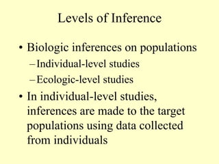
15. Ecological Fallacy
• Assumptions:
–1) that the effects estimated at the
individual level are the relevant ones
for making biological inferences
–2) that the effects are a linear
function of the predictors; i.e. E[yi] =
 + xi

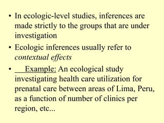
16. • Assume the above relationship {E[yi] =
 + xi} to hold on an individual level
and that the parameter of interest for
the purposes of biological inference is
.
• Assume now that the population is
segregated into groups and that the
analysis proceeds by comparing the
grouped mean between the k groups
(no individual data available).

17. • The slope including group effects is:
•  = G +  W
• where  is the overall between-
person slope (i.e., over all persons in
all groups), G is the between-group
slope (ecological effect), W is the
within-group slope, and ,  are ratios
of the between-group and within-group
variances to the total variance of x ( +
 =1).

18. • When there are no group effects then 
= W, so W is the correct regression
coefficient
• When there are group effects   W ,
so that G  W
• Ecological bias or “cross-level bias”
occurs when G  W
• See Piantadosi, AJE 1988;127:893-904

19. Conditions for No Ecological Bias
• Background rate of disease (in the
unexposed) does not vary across groups
– background rates may vary, apart from
statistical variation, due to unequal
distributions of risk factors across groups
– AND
• These is no confounding within groups
• AND
• There is no effect modification by group

20. • In general, the ecological linear regression
model will estimate the difference in rates
between groups.
• The ecological regression coefficient is
equal to the sum of:
– difference in rates at the individual level
– bias from the association between the
confounding factor and group
– bias from the interaction between a factor and
group (only if the difference in rates does not
vary by group will there be no interaction)

21. Examples of Ecological Bias
• Group is an effect modifier
– i.e., effect of exposure varies across
groups
– can arise from differential distribution of
effect modifiers across groups
– can occur even if after control for
ecological covariates

22. Ecological Bias: Effect Modification by Group, No Confounding
Eoesophageal cancer and smoking
Individual Level Analysis
Region 1 Region 2 Region 3 Total
Smoking Yes No Yes No Yes No Yes No
No of cases 13 3 12 3.6 12 4.2 36 10.8
Population 100000.100000. 80000.120000. 60000.140000. 240000.360000.
Rate/ 100.000 12 3 15 3 20 3 15 3
Rate ratio 4 5 6.7 5
Rate difference 9 12 17 12
Overall SMR 5 (Standardized to non-smokers; i.e., no confounding by grou
no confounging by group
Ecological Level Analysis
% smokers 0.5 0.4 0.3
Cancer rate 7.5 7.8 8.1

23. Confounding by Non-
Confounders
• Variable is not a confounder on the
individual level
–may occur if background rates vary
by group
–if rate differences between groups
not constant

24. Ecological Bias: Ecological Confounding of a non-Confounder
on the Individual Level
Lung cancer and radon
Individual Level Analysis
Region 1 Region 2 Region 3
Smokers Nonsmokers
Smokers Nonsmokers
Smokers Nonsmoker
Radon level Yes No Yes No Yes No Yes No Yes No Yes No
No of cases 52 74 5.2 7.4 56 52 8.4 7.8 60 30 14 7
Population
(in thousands) 26 74 26 74 28 52 42 78 30 30 70 70
Rate per 100,000 200 100 20 10 200 100 20 10 200 100 20 10
Rate by smoking level126 12.6 135 13.5 15 1.5
Rate ratio for smoking 10 10 10
Radon-smoking assocn. 1 1 1
Rate difference for radon
100 10 100 10 100 10
Rate ratio for radon 2 2 2 2 2 2

25. Adjustment for Ecological
Confounder Increases Bias
• Variable is not a confounder on the
individual level (factors not
associated)
–background rates differ by group
–rate differences vary by group

26. Ecological Bias: Ecological Confounder Increases Bias
Eoesophageal cancer and alcohol
Individual Level Analysis
Region 1 Region 2 Region 3
Smokers Nonsmokers
Smokers Nonsmokers
Smokers Nonsmokers
Alcohol Yes No Yes No Yes No Yes No Yes No Yes No
No of cases 13 2.5 1.5 0.7 14.7 1.1 1.1 1 15 0.6 1.9 0.9
Population
(in thousand
50 50 30 70 58.8 21 21 98.8 60 12 38 90
Rate per 100,000 25 5 5 1 25 5 5 1 25 5 5 1
Rate by smoking level
15 2.2 19.7 1.8 21.7 2.2
RR: smoking 6.6 11 9.9
Alc-smk assocn. 2.3 12.1 11.8
Rate diff.: alcohol 20 4 20 4 20 4
RR: alcohol 5 5 5 5 5 5

27. Nondifferential Misclassification
of Exposure
• For both linear and log-linear models
nondifferential misclassification of
exposure (binary variable) leads to an
overestimation of effect in ecological
studies, even if there are no other
sources of ecological bias
• See Brenner AJE 1992;135:85-95

28. Non-Linear Effects of Covariates
• If there is a nonlinear association
between the outcome, the exposure and
the covariate, ecological bias may occur
– due to the linear ecological model not
holding in the underlying population (e.g.,
Risk(x,c) = (1 + ßx) exp(c))
– not correctly summarizing the ecological
covariates across groups (using just means
instead of other more complex summaries)

29. Possible Solutions
• Obtain detailed information on
covariates so that not just mean levels
are used in the analysis
• Obtain joint distributions of covariates
and exposures
• Use another analytic approach
(individual-level or semi-individual-
level studies)

30. Example: Association between
Radon in Homes and Lung Cancer
• Studies of uranium miners and smelters have
shown strong positive exposure-response
relationships between level of radon gas and
lung cancer
• Ecological studies of lung cancer rates and
mean level of radon by county in the US and
elsewhere have shown strong negative
correlations

31. Case-control Study in Sweden
• 1360 cases and 2847 controls
• Age 35-74 years, 1980-84, living in 109
municipalities
• Radon monitored in 9000 homes occupied
by subjects since 1947 for > 2 years
• Time-weighted concentrations estimated per
subject
• Carried out an analysis of individual data
and ecological data

32. • Ecological radon levels: Average
radon exposure aggregated in each
municipality from controls living there
• Ecological analysis: Odds ratios per
county calculated (only males with >10
cases per county)

33. Ecological Association of Lung
Cancer and Radon by County,
Sweden
0
0,2
0,4
0,6
0,8
1
1,2
1,4
1,6
1,8
0 50 100 150 200
Estimated radon levels in controls
Odds
ratios
tios
.
1.8
1.6
1.4
1.2
0.8
0.6
0.4
0.2

34. Association of Radon and Lung Cancer Risk:
Comparison of Individual and Ecological Estimates
Regression Individual level Ecological
Model RR 95%CI RR 95%CI
Age, sex, urbanization, occupation 1.10.99-1.15 1 0.79-1.17
Plus: Individual smoking 1.10.98-1.13
Plus: Aggregated smoking 1 0.79-1.17
Plus: Individual smoking and latitude 1.11.02-1.24
Plus: Aggregated smoking and latitude 1.1 0.80-1.29
RR calculated per 100 Bq-cubic metre
Source: Lagarde and Pershagen AJE 1999;149:268-74.

35. References
• ECOLOGICAL STUDIES
• Chapter 23, “Ecological Studies”, Hal
Morgenstern, in Rothman and Greenland
• Richardson et al., Int J Epidem 1987;16:111-120.
• Piantadosi et al., Am J Epidem 1988;127:893-904.
• Greenland and Morgenstern, Int J Epidem
1989;18:269-274.
• Brenner et al., Am J Epidem 1992;135:85-95.
• Brenner et al., Epidemiology 1992;3:456-9.
• Greenland and Robbins, Am J Epidem
1994;139:747-760.