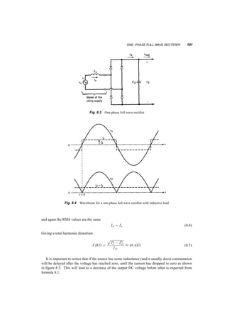
Downloaded 14 times


![2 THREE PHASE CIRCUITS AND POWER
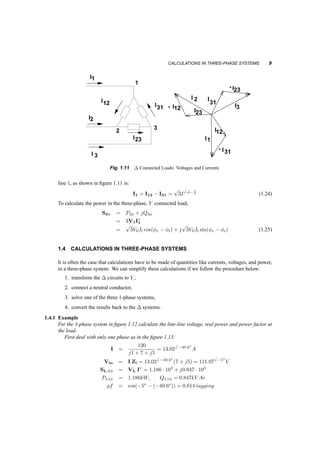
where i(t) is the instantaneous value of current through the load and v(t) is the instantaneous value
of the voltage across it.
In quasisteady
state conditions, the current and voltage are both sinusoidal, with corresponding
amplitudes^i
and ^v, and initial phases, Ái and Áv, and the same frequency, ! = 2¼=T ¡ 2¼f:
v(t) = ^v sin(!t + Áv) (1.2)
i(t) = ^i
sin(!t + Ái) (1.3)
In this case the rms values of the voltage and current are:
V =
s
1
T
Z T
0
^v [sin(!t + Áv)]2 dt =
^v
p
2
(1.4)
I =
s
1
T
Z T
0
^i
[sin(!t + Ái)]2 dt =
^i
p
2
(1.5)
and these two quantities can be described by phasors, V = V
6 Áv and I = I
6 Ái .
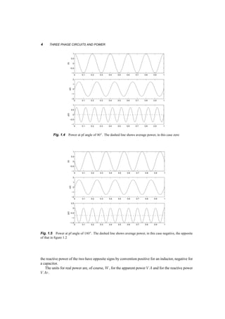
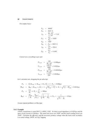
Instantaneous power becomes in this case:
p(t) = 2V I [sin(!t + Áv) sin(!t + Ái)]
= 2V I
1
2
[cos(Áv ¡ Ái) + cos(2!t + Áv + Ái)] (1.6)
The first part in the right hand side of equation 1.6 is independent of time, while the second part
varies sinusoidally with twice the power frequency. The average power supplied to the load over
an integer time of periods is the first part, since the second one averages to zero. We define as real
power the first part:
P = V I cos(Áv ¡ Ái) (1.7)
If we spend a moment looking at this, we see that this power is not only proportional to the rms
voltage and current, but also to cos(Áv ¡ Ái). The cosine of this angle we define as displacement
factor, DF. At the same time, and in general terms (i.e. for periodic but not necessarily sinusoidal
currents) we define as power factor the ratio:
pf = P
V I
(1.8)
and that becomes in our case (i.e. sinusoidal current and voltage):
pf = cos(Áv ¡ Ái) (1.9)
Note that this is not generally the case for nonsinusoidal
quantities. Figures 1.2 1.5
show the cases
of power at different angles between voltage and current.
We call the power factor leading or lagging, depending on whether the current of the load leads
or lags the voltage across it. It is clear then that for an inductive/resistive load the power factor is
lagging, while for a capacitive/resistive load the power factor is leading. Also for a purely inductive
or capacitive load the power factor is 0, while for a resistive load it is 1.
We define the product of the rms values of voltage and current at a load as apparent power, S:
S = V I (1.10)](https://image.slidesharecdn.com/ece320-notes-part12-140914210816-phpapp02/85/Ece320-notes-part1-2-10-320.jpg)
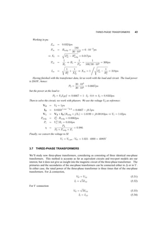
![6 THREE PHASE CIRCUITS AND POWER
We also notice that if for a load we know any two of the four quantities, S, P, Q, pf, we can
calculate the other two, e.g. if S = 100kV A, pf = 0:8 leading, then:
P = S ¢ pf = 80kW
Q = ¡S
q
1 ¡ pf2 = ¡60kV Ar ; or
sin(Áv ¡ Ái) = sin [arccos 0:8]
Q = S sin(Áv ¡ Ái)
Notice that here Q 0, since the pf is leading, i.e. the load is capacitive.
Generally in a system with more than one loads (or sources) real and reactive power balance, but
not apparent power, i.e. Ptotal =
P
i Pi, Qtotal =
P
i Qi, but Stotal6=
P
i Si.
In the same case, if the load voltage were VL = 2000V , the load current would be IL = S=V
= 100 ¢ 103=2 ¢ 103 = 50A. If we use this voltage as reference, then:
V = 20006 0V
I = 506 Ái = 506 36:9o
A
S = V I¤ = 20006 0 ¢ 506 ¡36:9o = P + jQ = 80 ¢ 103W ¡ j60 ¢ 103V Ar
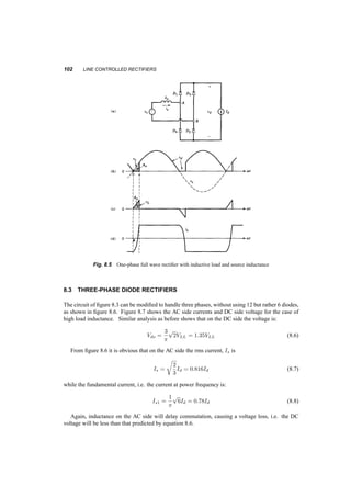
1.3 THREEPHASE
BALANCED SYSTEMS
Compared to single phase systems, threephase
systems offer definite advantages: for the same power
and voltage there is less copper in the windings, and the total power absorbed remains constant rather
than oscillate around its average value.
Let us take now three sinusoidalcurrent
sources that have the same amplitude and frequency, but
their phase angles differ by 1200. They are:
i1(t) =
p
2I sin(!t + Á)
i2(t) =
p
2I sin(!t + Á ¡
2¼
3
) (1.18)
i3(t) =
p
2I sin(!t + Á +
2¼
3
)
If these three current sources are connected as shown in figure 1.7, the current returning though node
n is zero, since:
sin(!t + Á) + sin(!t ¡ Á +
2¼
3
) + sin(!t + Á +
2¼
3
) ´ 0 (1.19)
Let us also take three voltage sources:
va(t) =
p
2V sin(!t + Á)
vb(t) =
p
2V sin(!t + Á ¡
2¼
3
) (1.20)
vc(t) =
p
2V sin(!t + Á +
2¼
3
)
connected as shown in figure 1.8. If the three impedances at the load are equal, then it is easy
to prove that the current in the branch n ¡ n0 is zero as well. Here we have a first reason why](https://image.slidesharecdn.com/ece320-notes-part12-140914210816-phpapp02/85/Ece320-notes-part1-2-14-320.jpg)


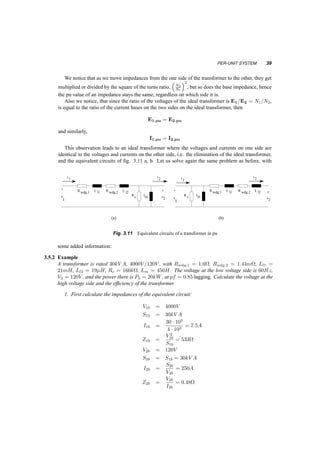
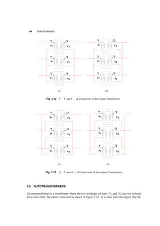
![40 TRANSFORMERS
2. Convert everything to per unit: First the parameters:
Rwdg;1;pu = Rwdg;1=Z1b = 0:003 pu
Rwdg;2;pu = Rwdg;2=Z2b = 0:003 pu
Xl1;pu =
2¼60Ll1
Z1b
= 0:015 pu
Xl2;pu =
2¼60Ll2
Z2b
= 0:0149 pu
Rc;pu = Rc
Z1b
= 300 pu
Xm;pu =
2¼60Llm
Z1b
= 318pu
Then the load:
V2;pu = V2
V2b
= 1pu
P2;pu = P2
S2b
= 0:6667pu
3. Solve in the pu system. We’ll drop the pu symbol from the parameters and variables:
I2 =
µ
P2
V2 ¢ pf
¶6 arccos(pf)
= 0:666 ¡ j0:413pu
V1 = V2 + I [Rwdg;1 + Rwdg;2 + j(Xl1 + Xl2)] = 1:0172 + j0:0188pu
Im =
V1
Rc
+
V1
jXm
= 0:0034 ¡ j0:0031pu
I1 = Im + I2 = 0:06701 ¡ j0:416 pu
Pwdg = I2
2 (Rwdg;1 + Rewg;2) = 0:0037 pu
Pcore = V 2
1
Rc
= 0:0034pu
´ = P2
Pwdg + Pcore + P2
= 0:9894
4. Convert back to SI. The efficiency, ´, is dimensionless, hence it stays the same. The voltage,
V1 is
V1 = V1;puV1b = 40696 10
V
3.6 TRANSFORMER TESTS
We are usually given a transformer, with its frequency, power and voltage ratings, but without the
values of its impedances. It is often important to know these impedances, in order to calculate voltage
regulation, efficiency etc., in order to evaluate the transformer (e.g. if we have to choose from many)
or to design a system. Here we’ll work on finding the equivalent circuit of a transformer, through
two tests. We’ll use the results of these test in the perunit
system.
First we notice that if the relative values are as described in section 3.4, we cannot separate the
values of the primary and secondary resistances and reactances. We will lump R1;wdg and R2;wdg](https://image.slidesharecdn.com/ece320-notes-part12-140914210816-phpapp02/85/Ece320-notes-part1-2-49-320.jpg)

![4
Concepts of Electrical
Machines; DC motors
DC machines have faded from use due to their relatively high cost and increased maintenance
requirements. Nevertheless, they remain good examples for electromechanical systems used for
control. We’ll study DC machines here, at a conceptual level, for two reasons:
1. DC machines although complex in construction, can be useful in establishing the concepts of
emf and torque development, and are described by simple equations.
2. The magnetic fields in them, along with the voltage and torque equations can be used easily to
develop the ideas of field orientation.
In doing so we will develop basic steadystate
equations, again starting from fundamentals of the
electromagnetic field. We are going to see the same equations in ‘Brushless DC’ motors, when we
discuss synchronous AC machines.
4.1 GEOMETRY, FIELDS, VOLTAGES, AND CURRENTS
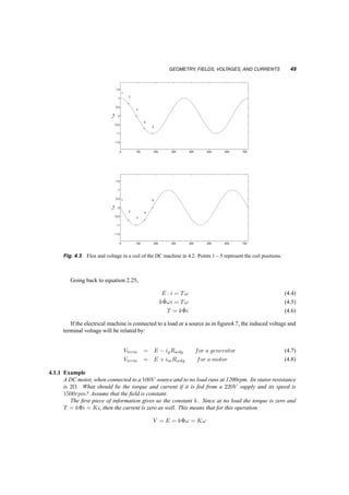
Let us start with the geometry shown in figure 4.1
This geometry describes an outer iron window (stator), through which (i.e. its center part) a
uniform magnetic flux is established, say ^©. How this is done (a current in a coil, or a permanent
magnet) is not important here.
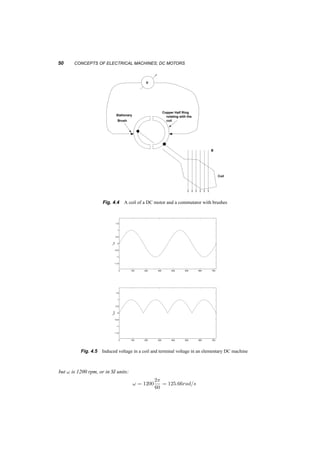
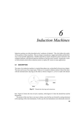
In the center part of the window there is an iron cylinder (called rotor), free to rotate around its
axis. A coil of one turn is wound diametrically around the cylinder, parallel to its axis. As the
cylinder and its coil rotate, the flux through the coil changes. Figure 4.2 shows consecutive locations
of the rotor and we can see that the flux through the coil changes both in value and direction. The
top graph of figure 4.3 shows how the flux linkages of the coil through the coil would change, if the
rotor were to rotate at a constant angular velocity, !.
¸ = ^©
cos [!t] (4.1)
47](https://image.slidesharecdn.com/ece320-notes-part12-140914210816-phpapp02/85/Ece320-notes-part1-2-56-320.jpg)
![5
Threephase
Windings
Understanding the geometry and operation of windings in AC machines is essential in understanding
how these machines operate. We introduce here the concept of Space Vectors, (or Space Phasors) in
its general form, and we see how they are applied to threephase
windings.
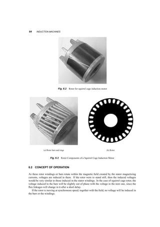
5.1 CURRENT SPACE VECTORS
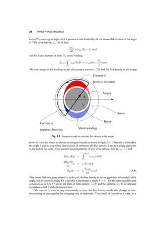
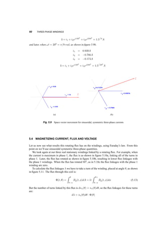
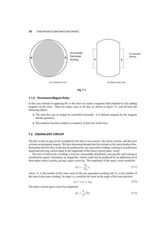
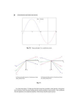
Let us assume that in a uniformly permeable space we have placed three identical windings as shown
in figure 5.1. Each carries a time dependent current, i1(t), i2(t) and i3(t). We require that:
i1(t) + i2(t) + i3(t) ´ 0 (5.1)
Each current produces a flux in the direction of the coil axis, and if we assume the magnetic
medium to be linear, we can find the total flux by adding the individual fluxes. This means that we
could produce the same flux by having only one coil, identical to the three, but placed in the direction
of the total flux, carrying an appropriate current. Figure 5.2 shows such a set of coils carrying for
i1 = 5A, i2 = ¡8A and i3¡ = 3A and the resultant coil.
To calculate the direction of the resultant one coil and the current it should carry, all we have to
do is create three vectors, each in the direction of one coil, and of amplitude equal to the current of
each coil. The sum of these vectors will give the direction of the total flux and hence of the one coil
that will replace the three. The amplitude of the vectors will be that of the current of each coil.
Let us assume that the coils are placed at angles 00, 1200 and 2400. Then their vectorial sum will
be:
i = i
6 Á = i1 + i2ej1200 + i3ej2400 (5.2)
We call i, defined thus, a space vector, and we notice that if the currents i1, i2 and i3 are functions
of time, so will be the amplitude and the angle of i. By projecting the three constituting currents on
the horizontal and vertical axis, we can find the real (id = [i]) and imaginary (iq = =[i]) parts of
53](https://image.slidesharecdn.com/ece320-notes-part12-140914210816-phpapp02/85/Ece320-notes-part1-2-62-320.jpg)
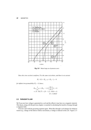
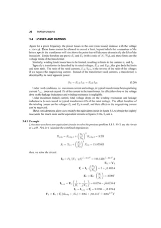
![54 THREEPHASE
WINDINGS
I
3
3
F 2
F
2
I
I
1
1
F
Fig. 5.1 Three phase concentrated windings
-8A
3A
5A
-8A
(a)
3A
5A
__
2 I
__
I
__
I1
3
__
I
(b)
5A
3A
-8A
F
I1
I2
I3
I
I
F
(c)
Fig. 5.2 Currents in three windings (a), Resultant space vector (b), and corresponding winding position (c)
it. Also, from the definition of the current space vector we can reconstruct the constituent currents:
i1(t) =
2
3
[i(t)]
i2(t) =
2
3
[i(t)e¡j°] (5.3)
i3(t) =
2
3
[i(t)e¡j2°]
° = 1200 =
2¼
3 rad (5.4)](https://image.slidesharecdn.com/ece320-notes-part12-140914210816-phpapp02/85/Ece320-notes-part1-2-63-320.jpg)

![78 INDUCTION MACHINES
while the previously developed formulas for maximum torque will become:
Tmax = 3p
2
1
2!s
V 2
Th
RTh +
q
R2T
h + (XTh + Xlr)2
(6.32)
and
Tmax '
3
2
p
2
µ
Vs
!s
¶2 1
RR
(!s ¡ !Tmax) =
3
2
p
2
µ
Vs
!s
¶2 1
Lls + Llr
(6.33)
6.8.1 Example
A 3phase
2pole
induction motor is rated 190V , 60Hz, it is connected in Y , and has Rr = 6:6,
Rs = 3:1, XM = 190, Xlr = 10, and Xls = 3. Calculate the motor starting torque, starting
current and starting power factor under rated voltage. What will be the current and power factor if
no load is connected to the shaft?
1. At starting s = 1:
Is =
190
p
3
= f[3:1 + j3] + j190jj(6:6 + j10)g = 7:066 ¡54:50
A
IR = Is
j190
6:6 + j10 + j190
= 6:76 ¡52:60
A
T = 3Pgap
!s
p
2
= 3
6:72 ¢ 6:6
377
2
2
= 2:36Nm
2. Under no load the speed is synchronous and s = 0:
Is = 110= [3:1 + j3 + j190] = 0:576 ¡89:10
A
Is = 0:57A
pf = 0:016lagging
6.8.2 Example
A 3phase
2pole
induction motor is rated 190V , 60Hz it is connected in Y , and has Rr = 6:6,
Rs = 3:1, XM = 190, Xlr = 10, and Xls = 3. It is operating from a variable speed variable
frequency source at a speed of 1910rpm, under a constant V=f policy and the developed
torque is 0:8Nm. What is the voltage and frequency of the source? (Hint: Calculate first the slip).
The ratio Vs=!s stays 110=377.
T = p
2
3
µ
Vs
!s
¶2 1
RR
!r
0:8 = 1 ¢ 3
µ
110
377
¶2 1
6:6!r ) !r = 20:65 rad/s
!s = !m
p
2
+ !R = 220:66 rad
s
) fs = 35Hz ) Vs = 220:66
110
377
= 64:4V or 110Vl¡l
6.8.3 Example
A 3phase
4pole
induction machine is rated 230V , 60Hz. It is connected in Y and it has Rr =
0:191, Rs = 0:2, LM = 35mH, Llr = 1:5mH, and Lls = 1:2mH. It is operated as a generator](https://image.slidesharecdn.com/ece320-notes-part12-140914210816-phpapp02/85/Ece320-notes-part1-2-87-320.jpg)
![MULTIPLE POLE PAIRS 79
connected to a variable frequency/variable voltage source. Its speed is 2036rpm, with countertorque
of 59Nm. What is the efficiency of this generator? (Hint: here power in is mechanical, power out
is electrical; calculate first the slip)
Although we do not know the voltage or the frequency, we know their ratio since it is always
132:8=377.
T = 3p
2
µ
Vs
!s
¶2 1
RR
!r
) ¡59 = 3 ¢ 2
µ
132:8
377
¶2 1
0:191!r
) !r = ¡15:14 rad/s
Now we can find the synchronous speed, by adding slip and rotor speeds:
!s = !m
p
2
+ !r =
2¼ ¢ 2036
60
2 ¡ 15:14 = 411:3 rad/s
) fs = 65:5Hz ) Vs = 65:5 ¢
132
60
= 144V
We have to recalculate the impedances of the equivalent circuit for the frequency of 65:5Hz:
Xm = 35 ¢ 10¡3 ¢ 411:3 = 14:4; Xls = 0:49; Xlr = 0:617
RR
!r + !m
p
2
!r
= ¡5:38
Is = 144= [0:2 + j0:49 + j14:4jj(0:191 ¡ 5:38 + j0:617)] = 306 ¡1480
A
IR = 27:26 ¡166:9A
Notice that with generation operation RR 0. We can calculate now losses etc.
Pm = 3 ¢ 27:225:38 = 11:941kW
Protor;loss = 3 ¢ 27:220:191 = 423W
Pstator;loss = 3 ¢ 3020:2 = 540W
) Pout = Pm ¡ Protor;loss ¡ Pstator;loss = 10:980kW
) ´ = Pout
Pm
= 0:919](https://image.slidesharecdn.com/ece320-notes-part12-140914210816-phpapp02/85/Ece320-notes-part1-2-88-320.jpg)
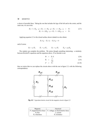
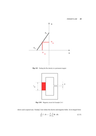
![90 SYNCHRONOUS MACHINES AND DRIVES
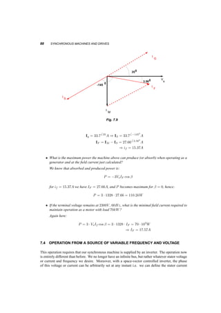
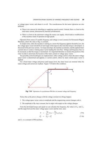
More common though is the case when the stator voltage is not constant. Here we monitor the
position of the rotor and since the rotor flux and rotor space current are attached to it, we are actually
monitoring the position of IF. To make matters simple we use this current rather than the stator
voltage as reference, as shown in figure 7.11.
I
V s
IM
F
I s
jI F X M
jI s X M
g
q
Fig. 7.11 Operation of a synchronous PM drive below base speed
Although previous formulae for power and torque are still true they are not as useful. We create
new formulae that have the stator current Is and magnetizing current IM as variables. We also use
the angle °, between IF and Is, since we can control it. Starting from what we already know:
Pg = [VsI¤
F] = [jXM(IF + Is)I¤
F] (7.11)
= [jXMIFI¤
F] + [jXMIsI¤
F] (7.12)
= XM=[IsI¤
F] = XMIsIF sin ° (7.13)
For a given torque minimum losses require minimum value of the stator current. To minimize the
value of Is with constant power and IF we choose ° = 90o and arrive at:
Pg = XM=[IsI¤
F] = XMIsIF (7.14)
T = 3p
2
Pg
!s
= 3p
F] = 3p
2LM=[IsI¤
2LMIsIF (7.15)
which means that for constant power the projection of the stator current on an axis perpendicular to
IM is constant.
As the rotor speed increases, even if IM stays constant, the stator voltage Vs = !sLmIs increases.
At some speed !sB, the required voltage exceeds the maximum the power source can provide. We
call this speed base speed; To increase the speed beyond it we no longer keep ° = 90o. On the other
hand at that speed we know that the voltage has reached its upper limit Vs = Vs;max, therefore the
value of IM = Vs;max=XM is known. In this case, equations 7.9 and 7.10 become:
T =
3p
2!s
VsIs cos µ =
3p
2 LMIMIs cos µ (7.16)
I2F
= I2M
+ I2
s + 2IMIs sin µ (7.17)](https://image.slidesharecdn.com/ece320-notes-part12-140914210816-phpapp02/85/Ece320-notes-part1-2-99-320.jpg)
![OPERATION FROM A SOURCE OF VARIABLE FREQUENCY AND VOLTAGE 91
I s1
I M2
jI F X M
jI s1 X M
V s1
jI s2 X M
q1
q2
V
I
g
g 1
2
M1
I
s2
s2
I
F
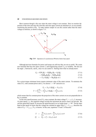
Fig. 7.12 Field weakening of a PM AC motor. The two diagrams at are at the same frequency, but the second
one has ° 90o and lower Vs
.
Figure 7.12 shows such an operation with the variables having the subscript 1. Note that we
calculate torque from power:
P = 3XMISIF sin ° (7.18)
T = P
!s
p
2
= 3p
F] = 3p
2LM=[ISI¤
2LMIsIF sin ° (7.19)
7.4.1 Example
A 3phase,
four pole, Y connected permanent magnet synchronous machine is rated 400V , 50Hz,
50kV A. Its magnetizing inductance is 2:5mH and its equivalent field source current is 310A. We
can neglect stator resistance.
² The machine is operated as a generator at rated frequency. Determine the maximum and
minimum values of the stator phase voltage as the load current is varied from zero to rated
value at unity power factor.
p
The rated phase voltage is Vs = 400=
3 = 231V and the rated stator current is Is =
50 ¢ 103=3 ¢ 231 = 72:2A. With no load and at rated frequency the phase voltage is:
Vs = !sLMIF = 2¼50 ¢ 2:5 ¢ 10¡3 ¢ 310 = 243:5V
If the motor is operated at unity power factor, the stator current is collinear with the stator
voltage, as in figure 7.13.
From the current triangle:
I2M
= I2F
s ) IM =
¡ I2
p
3102 ¡ 72:72 = 301:5A
and the stator voltage is:
Vs = !sLMIM = 236:8V
² The machine is now operated as a variable speed drive motor from a variable voltage, variable
frequency source. What should be the voltage and frequency in order to provide torque of
300Nm at 600rpm, if again we have unity power factor?](https://image.slidesharecdn.com/ece320-notes-part12-140914210816-phpapp02/85/Ece320-notes-part1-2-100-320.jpg)


This document provides an introduction to three-phase circuits and power calculations. It defines key concepts like real power, reactive power, apparent power and power factor for sinusoidal steady-state systems. It describes how to calculate power in single-phase and three-phase balanced systems using phasors. It also discusses power factor in lagging and leading configurations and how to determine the power factor from load characteristics.


![Electric drives [ned mohan 2001 (scanned) 470pág]](https://cdn.slidesharecdn.com/ss_thumbnails/electricdrivesnedmohan2001-scanned470pg-121224050928-phpapp01-thumbnail.jpg?width=640&height=640&fit=bounds)


