Download to read offline
![IOSR Journal of Mathematics (IOSR-JM)
e-ISSN: 2278-5728,p-ISSN: 2319-765X, Volume 7, Issue 3 (Jul. - Aug. 2013), PP 19-29
www.iosrjournals.org
www.iosrjournals.org 19 | Page
Statefinder Diagnostic for Binary Mixture of Anisotropic Dark
Energy and Perfect Fluid in Bianchi Type-IX Universe
H. R. Ghate1
, Atish S. Sontakke2
1,2
Department of Mathematics, Jijamata Mahavidyalaya, Buldana (India)-443001
Abstract : The new Bianchi type-IX cosmological models with binary mixture of perfect fluid and anisotropic
dark energy have been studied. The unique solution of field equations is obtained by assuming that the energy
conservation equation of the perfect fluid and dark energy vanishes separately together with a special law for
the mean Hubble parameter (Berman, 1983) which yields a constant value of the deceleration parameter and
generates two types of solutions, one is of power law type and other is of the exponential type. To have a general
description of an anisotropic dark energy component in terms of its equation of state
)(de
, a skewness
parameters have been introduced. The statefinder diagnostic pair (i.e. sr, parameter) is used to
characterize different phases of the universe. The various geometric and kinematic properties of the model and
the behavior of the anisotropy of the dark energy have been discussed.
Keywords - Anisotropic Dark Energy, Perfect Fluid, Bianchi type-IX Universe, Statefinder parameters.
I. Introduction
In 1998, two teams have independently studied distant type Ia Supernovae (SNe Ia) and observed that,
the universe is experiencing an accelerated expansion [1-2]. These remarkable findings were confirmed later
from the studies of supernovae and independent evidences from cluster of galaxies, large scale structure [3-4]
and the cosmic microwave background (CMB) [5-6]. In Einstein‟s general relativity, for such type of
acceleration, one needs to introduce a component to the matter distribution of the universe with a large negative
pressure. This component is usually referred as „Dark Energy‟ (DE). The DE occupies about 73% of the total
energy of the universe, while dark matter occupies 23% and the usual baryonic matter is 4%. DE is described
phenomenologicaly by an equation of state (EoS) p where p and are the pressure and energy
density of DE and is an EoS parameter which is useful to describe cosmic acceleration. A number
of authors [7-15] have studied binary mixture of perfect fluid (PF) and anisotropic DE for Bianchi type-I, II, III,
V, VI0, plane symmetric, kaluza-klein as well as higher dimensional cosmological models too. Recently, the
anisotropic dark energy has been studied for Bianchi type-IX space-time [16].
The theoretical arguments and recent experimental data supports the existence of an anisotropic phase
that approaches anisotropy. This is because we consider models of the universe with an anisotropic background.
Bianchi type homogeneous models are the simplest of the anisotropic models. These models also used to
examine the role of certain anisotropic sources during the formation of the large scale structure as we see in the
universe today. Bianchi type-IX cosmological models are very popular for relativistic studies. They have
solutions of type Robertson-Walker universe with positive curvature, the de-Sitter universe and Taub-NUT
solutions. These models are not only anisotropic but also allow expansion, rotation and shear. Many authors [16-
25] have studied different aspects of Bianchi type-IX cosmological models in various theories of gravitation.
Recently, Bianchi type-IX DE model in Brans-Dicke theory of gravitation has been studied [26].
In the last few years, high red-shift supernova experiments had dramatically increased the quality of
cosmological observational data. There are many DE models proposed recently to explain the cosmic
acceleration. From the observations, we see that there is a variation in the properties of DE depending on the
cosmological model. In order to differentiate among different forms of DE, Sahni et al. [27] proposed a new
geometrical diagnostic pair of statefinders parameters sr, which are defined as
3
RH
R
r
and
213
1
q
r
s , (1)
Where H is the Hubble parameter, R is an average scale factor and q is the deceleration parameter.
The parameter r forms the next step in the hierarchy of geometrical cosmological parameters after the Hubble
parameter H and the deceleration parameter q , while s is a linear combination of q and r chosen in such a
way that it does not depend upon the DE density. The statefinder pair is calculated for a number of existing](https://image.slidesharecdn.com/e0731929-150428030241-conversion-gate01/75/E0731929-1-2048.jpg)
![Statefinder Diagnostic for Binary Mixture of Anisotropic Dark Energy and Perfect Fluid in Bianchi
www.iosrjournals.org 20 | Page
models of DE [28-38] having both constant and variable . Hence, we are motivated to study Bianchi type-IX
DE model using this method of Statefinder diagnostic.
In the present paper, we have investigated new Bianchi type-IX cosmological models with binary
mixture of anisotropic DE and perfect fluid. The statefinder diagnostic pair sr, is adopted to characterize
different phases of the universe. The geometrical and physical behaviors of the model are also discussed.
II. Metric And The Field Equations:
Bianchi type-IX metric is considered in the form
ydxdzadzyaybdybdxadtds cos2cossin 222222222222
, (2)
where ba, are scale factors and are functions of cosmic time t .
The model has one transverse direction x , and two equivalent longitudinal directions y and z . In
natural units ( 1,18 cG ), Einstein‟s field equations in case of a binary mixture of PF and anisotropic DE
components are
ji
ed
ji
fp
jijiji TTRgRG
2
1
, (3)
with
)()()()(
,,, fpfpfpfpj
i
fp
pppdiagT
)()()()(
,,,1 fpfpfpfp
diag , (4)
and
)()()()(
,,, ed
z
ed
y
ed
x
edj
i
ed
pppdiagT
)()()()(
,,,1 eded
z
ed
y
ed
xdiag ,
)()()()(
)(),(,,1 edededed
diag , (5)
where, jig is the metric potentials with 1ji
ij uug ;
i
u is the flow vector; jiR is the Ricci tensor;
R is the Ricci scalar;
)( fp
and
)( ed
are the energy densities of PF and DE components respectively;
)( fp
is the EoS parameter of PF with 0)(
fp
and
)( ed
is the EoS parameter of DE;
)( ed
x ,
)( ed
y and
)( ed
z are the deviation-free EoS parameter of the DE on the x , y and z axes, respectively. is the
deviation-free EoS parameters of the DE. Here and are not necessarily constants and can be function of
the cosmic time t .
The Einstein‟s field equations (3) for metric (2) with the help of equations (3) and (5) can be written as
)()(
4
2
22
2
4
1
2 edfp
b
a
bb
b
b
b
a
a
(6)
)()()()(
4
2
22
2
4
31
2 ededfpfp
b
a
bb
b
b
b
(7)
)()()()(
4
2
)(
4
ededfpfp
b
a
b
b
a
a
b
b
a
a
, (8)
where over dot () denotes the differentiation with respect to t .
The Bianchi identity is given by
0;;; ji
j
edji
j
fpji
j TTG (9)
This yields:
022121 )()()()()()()(
b
b
b
b
a
a
b
b
a
a ededededfpfpfp
.
(10)
The directional Hubble parameters in the directions of x, y and z axes for the metric (2) are defined as
a
a
Hx
,
b
b
HH zy
. (11)](https://image.slidesharecdn.com/e0731929-150428030241-conversion-gate01/75/E0731929-2-2048.jpg)
![Statefinder Diagnostic for Binary Mixture of Anisotropic Dark Energy and Perfect Fluid in Bianchi
www.iosrjournals.org 21 | Page
The mean Hubble parameter is
b
b
a
a
V
V
H
2
3
1
3
1
, (12)
where the spatial volume of the universe is
2
abV . (13)
The anisotropy of the expansion can be parameterized after defining the directional Hubble parameters
and the mean Hubble parameter of the expansion.
The anisotropic parameter of the expansion is defined as
23
13
1
H
HHi
i
,
(14) where iH 3,2,1i represent the directional Hubble parameters in the directions of x, y and z
respectively. 0 corresponds to isotropic expansion. The space approaches isotropy, in case of diagonal
energy momentum tensor ( 00
i
T , where 3,2,1i ) if 0 , V and 000
T 0 as
t (Collins and Hawking, 1973).
Using equations (11) and (12,) equation (14) simplifies to
2
2
9
2
yx HH
H
, (15)
where yx HH is the difference between the expansion rates on x and y axes which can be
obtained by using the field equations.
On subtracting (7) from equation (8), we obtain
Vdt
b
ab
VVb
b
a
a
HH ed
yx
)(
4
22
1
, (16)
where is a constant of integration and the term with arises due to the possible intrinsic anisotropy
of the fluid.
To obtain the anisotropy parameter of the expansion, using (16) in (15), we get
2
2
)(
4
22
2
9
2
VVdt
b
ab
H
ed
. (17)
Choosing =0, the anisotropy parameter of the expansion for a Bianchi type-IX cosmological model
in the presence of PF reduces to
2
2
4
22
2
9
2
VVdt
b
ab
H
. (18)
The integral term in (17) vanishes for
4)(
22
b
ab
ed
. (19)
The energy momentum tensor (5) for anisotropic DE becomes
)(
4)(
22
)(
4)(
22
)()(
,,,1 ed
ed
ed
ed
ededj
i
b
ab
b
ab
diagT
. (20)
Using (19) in equation (17), the anisotropic parameter of the expansion reduces to
2
2
2
9
2
V
H
. (21)
It is seen that the above anisotropic parameter of the expansion is exactly same for exponential
expansion with anisotropic fluid [16, 33] and is equivalent to ones obtained for exponential expansion with
isotropic fluid [39-40].
The vanishing of the integral term also reduces the difference between the expansion rates on x and y
to the following form](https://image.slidesharecdn.com/e0731929-150428030241-conversion-gate01/75/E0731929-3-2048.jpg)
![Statefinder Diagnostic for Binary Mixture of Anisotropic Dark Energy and Perfect Fluid in Bianchi
www.iosrjournals.org 22 | Page
2
abV
HH yx
. (22)
Using equations (19) and (20) in the Einstein‟s field equations (6-8), one can obtain the reduced field
equations as
)()(
4
2
2
2
)1(
4
3
2 edfp
b
a
b
b
ba
ba
(23)
)()()()(
4
2
22
2
4
31
2 ededfpfp
b
a
bb
b
b
b
(24)
)()()()(
4
2
2
4
31 ededfpfp
b
a
bb
b
a
a
b
b
a
a
. (25)
III. Solutions Of The Field Equations:
Now we have, three linearly independent equations (23-25) and six unknown functions a , b ,
)( fp
,
)( ed
,
)( fp
,
)( ed
. Hence, we need three extra equations to solve the system completely.
Firstly, we assume that the DE and PF is minimally interacting (Adhav [33]) i.e.
0; ji
j
fp
T and 0; ji
j
ed
T
Hence, the Bianchi identity (10) can be split into two separately additive conserved components.
Therefore, the conservation equation of energy momentum tensor of DE and PF becomes
0221 )()()()(
;
b
b
b
b
a
a
T ededededji
j
ed
. (26)
021 )()()(
;
b
b
a
a
T fpfpfpji
j
fp
. (27)
Secondly, we assume that the EoS parameter of the PF to be constant i.e.
)(
)(
)(
fp
fp
fp p
= constant. (28)
Lastly, we use respectively the exponential volumetric expansion law as
kt
eCV 3
1 , (29)
and the power law volumetric expansion as
m
tCV 3
1 , (30)
where 1C , k and m are positive constants.
For 1m , the model exhibits accelerating volumetric expansion, on the other hand for 1m , the
model exhibits volumetric expansion with constant velocity whereas for 1m , the model exhibits decelerating
volumetric expansion. The anisotropic fluid we take here can be considered in the context of DE in the model
with exponential expansion and power law expansion for 1m .
IV. Model For Exponential Expansion V=C1e3kt
:
The scale factors a and b are obtained by solving the field equations (23-25) for the exponential
volumetric expansion (29) by considering (22),
)
9
2
exp( 3
1
3
1
2
21
kt
e
kC
ktCCa
,
(31) )
9
1
exp( 3
1
3
1
2
1 kt
e
kC
kt
C
C
b
, (32)
where 2C is a positive constant of integration.
The mean Hubble parameter is given by](https://image.slidesharecdn.com/e0731929-150428030241-conversion-gate01/75/E0731929-4-2048.jpg)
![Statefinder Diagnostic for Binary Mixture of Anisotropic Dark Energy and Perfect Fluid in Bianchi
www.iosrjournals.org 23 | Page
kH . (33)
The directional Hubble parameters on the x, y and z axes are respectively are given by,
kt
x e
C
kH 3
13
2
and
kt
zy e
C
kHH 3
13
1
. (34)
Using equations (33), (34) in equation (15), the anisotropic parameter of the expansion becomes,
kt
e
Ck
6
2
1
2
2
9
2
. (35)
It is observed that the above anisotropic parameter of the expansion is exactly same for exponential
expansion with anisotropic fluid [16, 33] and is equivalent to ones obtained for exponential expansion with
isotropic fluid [39-40].
Using equations (12) and (33) in equation (27), the energy density of the PF is found to be
tkfp fp
et )1(3
0
)( )(
)(
. (36)
From equation (36), it is observed that, the energy density of PF is constant at initial epoch and starts
decreasing with increase in time and becomes zero as t as shown in figure 1.
Using equations (31), (32) and (36) in equation (23), the energy density of the DE is found to be
tk
e
kC
kte
Ck
kt
kted fp
ktkt
ee
C
C
Ce
C
C
e
C
k )1(3
0
9
8
23
2
1
22
2
9
2
23
2
1
26
2
1
2
2)( )(
3
1
3
1
4
1
3
3
. (37)
From equation (37), the energy density of the DE is constant at initial epoch and starts decreasing with
increase in time. For large values of time t , the energy density of DE reduces to a fixed constant which matches
with the data from recent cosmological observations that the universe is accelerating as shown in figure 2.](https://image.slidesharecdn.com/e0731929-150428030241-conversion-gate01/75/E0731929-5-2048.jpg)
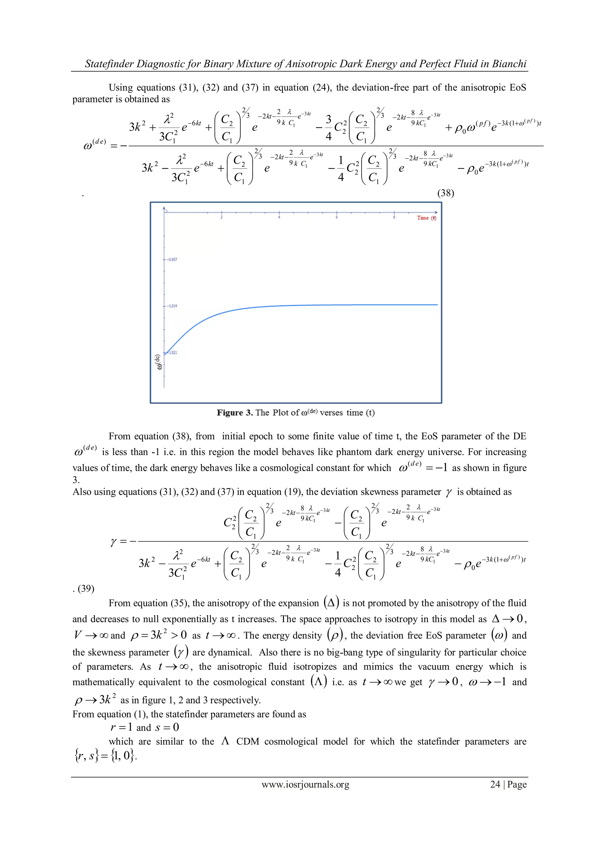
![Statefinder Diagnostic for Binary Mixture of Anisotropic Dark Energy and Perfect Fluid in Bianchi
www.iosrjournals.org 25 | Page
According to the conditions given by Collins and Hawking [41], the model isotropizes for large values
of t . Also, the anisotropy of the DE isotropizes for large values of t . This is consistent with the present day
observations that the universe is isotropic.
V. Model For Power Law Expansion m
tCV 3
1 :
The scale factors a and b are obtained by solving the field equations (23-25) for the Power Law
volumetric expansion (30) by considering (22),
m
t
Cm
m
etCCa 313
2
3
1
2
21
31
1
, (40)
m
t
Cm
m
et
C
C
b 313
3
1
2
1
31
1
, (41)
where 1C , 2C are positive constants of integration.
The mean Hubble parameter is
t
m
H . (42)
The directional Hubble parameters on the x, y and z axes are respectively are given by
m
x t
Ct
m
H 3
13
2
and
m
zy t
Ct
m
HH 3
13
1
. (43)
Using equations (42), (43) in equation (15), the anisotropic parameter of the expansion becomes,
2
62
2
1
2
9
2
m
t
C
m
. (44)
Using equations (12) and (42) in equation (27), the energy density of the PF is found to be
)1(3
0
)( )(
)(
fp
mfp
tt
. (45)
From equation (45), it is observed that, the energy density of PF )( pf
as 0t i.e. there is a
big-bang singularity and starts decreasing with increase in time and becomes zero as t as shown in fig. 4.
Using equations (40), (41) and (45) in equation (23), the energy density of the DE is found to be
)1(3
0
313
8
2
3
2
1
22
2
313
2
2
3
2
1
26
2
1
2
22 )(
31
1
31
1
4
1
3
3
fp
mm
mm
t
Cmm
t
Cmm
tet
C
C
Cet
C
C
t
C
tm
.
(46)](https://image.slidesharecdn.com/e0731929-150428030241-conversion-gate01/75/E0731929-7-2048.jpg)

![Statefinder Diagnostic for Binary Mixture of Anisotropic Dark Energy and Perfect Fluid in Bianchi
www.iosrjournals.org 27 | Page
Also using equations (40), (41) and (42) in equation (19), the deviation skewness parameter on z-
axis is obtained as
)1(3
0
313
8
2
3
2
1
22
2
313
2
2
3
2
1
26
2
1
2
22
313
2
2
3
2
1
2313
8
2
3
2
1
22
2
)(
31
1
31
1
31
1
31
1
4
1
3
3
fp
mm
mm
mm
t
Cmm
t
Cmm
m
t
Cmm
t
Cm
tet
C
C
Cet
C
C
t
C
tm
et
C
C
et
C
C
C
. (48)
From equation (42), it is observed that, the mean Hubble parameter H is infinitely large at 0t and reduces
for increasing values of t and becomes zero as t . The anisotropy of the expansion behaves
monotonically, decays to zero for 31m and diverges for 31m and is constant for 31m .
VI. Statefinder Diagnostic
In the last few years number of cosmologists have developed more number of DE models. To explain
the current cosmic acceleration the oldest and most familiar method is by observing the Hubble constant 0H and
the current value of the deceleration parameter 0q . Sahni et al. [ ] and Alam et al. [ ] have proposed a new
method to explain the current cosmic acceleration by introducing a cosmological diagnostic pair sr, which
they termed as statefinder. The two parameters are dimensionless and are geometrical since they are derived
from cosmic scale factors alone, though one can rewrite them in terms of the parameters of DE and DM. This
pair gives information about DE in a model-independent way i.e. it categorizes DE in the context of background
geometry only which is not dependent on theory of gravity. The statefinder parameters are depends upon the
expansion factor and hence upon the metric describing space and time. They can effectively differentiate
different forms of DE and provide simple diagnosis regarding whether a particular model fits into the basic
observational data. According to Sahni, the statefinder parameters sr, are defined as
3
)(
RH
R
tr
and
2
1
3
1
)(
q
r
ts
where H is the Hubble parameter, R is an average scale factor and q is the deceleration parameter.
In this letter, models for exponential expansion and power law expansion are discussed. In the former
model, we observed that the statefinder parameters are found as 1r and 0s which are similar to the
CDM cosmological model for which the statefinder parameters 0,1, sr indicating that the model
isotropizes for large values of t. Also the anisotropy of DE isotropizes for large value of t which are consistent
with the present day observations that the universe is isotropic. In the latter model the statefinder parameters are
found to be
23
)2)(1(
)(
m
mm
RH
R
tr
and
)2(3
)1(2
2
1
3
1
)(
m
rm
q
r
ts .](https://image.slidesharecdn.com/e0731929-150428030241-conversion-gate01/75/E0731929-9-2048.jpg)
![Statefinder Diagnostic for Binary Mixture of Anisotropic Dark Energy and Perfect Fluid in Bianchi
www.iosrjournals.org 28 | Page
Fig. 7 shows the variation of r against s for the values of .1,
2
1
,
3
1
m We observe that the model starts from
an Einstein Static Era sr , and goes to the CDM model 0,1 sr .
VII. Conclusion
The new Bianchi type-IX cosmological models is obtained with PF and anisotropic DE on the basis of
exponential expansion and power law expansion. In both the models the anisotropic DE isotropizes for large
values of t . The solution of the field equations are obtained by using special law for the mean Hubble parameter
(Berman, 1983) which yields a constant value of the deceleration parameter. The anisotropy of the space
isotropizes for exponential expansion. Also the anisotropy of the space isotropizes for power law expansion
model provided 31m . The statefinder diagnostic pair i.e. sr, parameter is adopted to characterize
different phases of the universe. It is observed that the exponential expansion model is similar to CDM
cosmological model for which the statefinder parameters are 0,1, sr . In case of power law expansion
model, the evolution trajectories in statefinder sr plane are plotted in figure 7. The power law expansion
model has the counters in the sr plane which shows the different phases of the universe. It is interesting to
note that our observations are analogous to the investigations of Akarsu and Kilinc [42] , Adhav [34] and Ghate
and Sontakke [16].
References
[1] S. Perlmutter et al., “Discovery of Supernovae explosion at half the age of the Universe”, Nature, Vol. 391, No. 2, pp. 51-54, 1998.
doi:10.1038/34124
[2] A. G. Reiss, et al., “Observational Evidence from super-novae for an Accelerating Universe and a Cosmological Constant,” The
Astrophysical Journal, Vol. 116, No. 3, 1998, pp. 1009-1038. doi:10.1086/300499.
[3] C. L. Benett et al., “First-Year Wilkinson Microwave Anisotropy Probe (WMAP) Observations: Preliminary Maps and Basic
Results”, Astrophys. J. Suppl. Ser., Vol. 148, No. 1, pp. 1, 2003. doi:10.1086/377253
[4] Hawkins S. et al., “The 2dF galaxy redshift survey: correlation functions, peculiar velocities and the matter density of the universe”,
Monthly Notices of the Royal Astronomical Society , Vol. 346 No. 1, pp. 78–96, 2003. doi.10.1046/j.1365-2966.2003.07063.x .
[5] R. R. CALDWELL, M. DORAN, “COSMIC MICROWAVE BACKGROUND AND SUPERNOVA CONSTRAINTS ON QUINTESSENCE:
CONCORDANCE REGIONS AND TARGET MODELS”, PHYSICS REVIEW D, VOL. 69, NO. 10, 103517, 2004. DOI.
10.1103/PHYSREVD.69.103517 .
[6] Z. Y. HUANG, B. WANG, E. ABDALLA, “HOLOGRAPHIC EXPLANATION OF WIDE-ANGLE POWER CORRELATION SUPPRESSION IN THE
COSMIC MICROWAVE BACKGROUND RADIATION” , JOURNAL OF COSMOLOGY AND ASTROPARTICLE PHYSICS, VOL. 2006, NO. 05,
DOI:10.1088/1475-7516/2006/05/013
[7] S. D. TADE, M. M. SAMBHE, “BIANCHI TYPE-I COSMOLOGICAL MODELS FOR BINARY MIXTURE OF PERFECT FLUID AND DARK
ENERGY”, ASTROPHYSICS AND SPACE SCIENCE, VOL. 338, PP. 179-185, 2012. DOI: 10.1007/S10509-011-0910-8
[8] S. KUMAR, O. AKARSU, “BIANCHI TYPE-II MODELS IN THE PRESENCE OF PERFECT FLUID AND DARK ENERGY”, THE EUROPEAN
PHYSICAL JOURNAL PLUS, VOL. 127, PP. 64, 2012. DOI: 10.1110/EPJP/I2012-12064-4
[9] S. D. KATORE ET AL., “BIANCHI TYPE-III COSMOLOGICAL MODEL WITH BINARY MIXTURE OF PERFECT FLUID AND DARK ENERGY”,
BULGARIAN JOURNAL OF PHYSICS, VOL. 38, PP. 390-399, 2011.
[10] T. SINGH, R. CHAUBEY, “BIANCHI TYPE-V COSMOLOGICAL MODELS WITH PERFECT FLUID AND DARK ENERGY”, ASTROPHYSICS AND
SPACE SCIENCE, VOL. 319, PP. 149-154, 2009. DOI: 10.1007/S10509-008-9959-4
[11] KATORE ET AL., “BIANCHI TYPE-VI0 COSMOLOGICAL MODELS WITH PERFECT FLUID AND DARK ENERGY”, INTERNATIONAL JOURNAL
OF THEORETICAL PHYSICS, VOL. 50, PP. 3299-3312, 2011B. DOI: 10.1007/S10773-011-0832-9
[12] S. D. KATORE, K. S. ADHAV, A. Y. SHAIKH, M. M. SANCHETI, “PLANE SYMMETRIC COSMOLOGICAL MODELS WITH PERFECT FLUID
AND DARK ENERGY”, ASTROPHYSICS AND SPACE SCIENCE, VOL. 333, PP. 333-341, 2011C. DOI: 10.1007/S10509-011-0622-0
[13] S. D. KATORE ET AL., “KALUZA-KLEIN COSMOLOGICAL MODEL FOR PERFECT FLUID AND DARK ENERGY”, BULGARIAN JOURNAL OF
PHYSICS, VOL. 40, PP. 17-32, 2013.
[14] K. S. Adhav et al., “Higher dimensional Bianchi type-I universe with perfect fluid and dark energy”, Bulgarian Journal of Physics,
Vol. 37, pp. 255-265, 2010.
[15] Adhav et al., “Higher dimensional Bianchi type-V cosmological models with perfect fluid and dark energy”, International Journal of
Theoretical Physics, Vol. 50, pp. 2573-2581, 2011. doi: 10.1007/s10773-011-0751-9
[16] H. R. Ghate, A. S. Sontakke, “Bianchi type-IX cosmological models with a anisotropic dark energy”, International Journal of
Scientific and Engineering Research, Vol. 4, No. 6, pp. 769-774, 2013.
[17] S. Chakraborty, “A study on Bianchi-IX cosmological model,” Astrophysics and Space Science, Vol. 180, No. 2, pp. 293–303,
1991. doi: 10.1007/BF00648184
[18] Shri Ram, Prem Singh, “Bianchi type-II, VIII and IX cosmological models with matter and electromagnetic fields”, Astrophysics
and Space Science, Vol. 201, No. 1, pp. 29-33, 1993. doi:10.1007/BF00626970
[19] K. S. Adhav et al., “Axially Symmetric Bianchi type-IX Inflationary Universe in General Relativity”, International Journal of
Theoretical Physics, Vol. 49, pp. 1753-1758, 2010. doi:10.1007/s10773-010-0355-9
[20] S.M.Waller, “Bianchi type IX electromagnetic universes”, Physical Review D., Vol. 29, No. 2, pp.176-185, 1984.
[21] R. Bali and S. Dave, “Bianchi Type-IX string cosmological model in general relativity,” Pramana, vol. 56, no. 4, pp. 513–518,
2001.
[22] R. Bali and M. K. Yadav, “Bianchi Type-IX viscous fluid cosmological model in general relativity,” Pramana Journal of Physics,
Vol. 64, No. 2, pp. 187–196, 2005. doi: 10.1007/BF02704873
[23] R. Bali, P. Kumawat, “Bianchi type IX stiff fluid tilted cosmological model with bulk viscosity”, European Journal of Theoretical
Physics, Vol. 7, No 24 , pp. 383-394, 2011.](https://image.slidesharecdn.com/e0731929-150428030241-conversion-gate01/75/E0731929-10-2048.jpg)
![Statefinder Diagnostic for Binary Mixture of Anisotropic Dark Energy and Perfect Fluid in Bianchi
www.iosrjournals.org 29 | Page
[24] A. Pradhan, S. K. Srivastav, and M. K. Yadav, “Some homogeneous Bianchi type IX viscous fluid cosmological models with a
varying Λ,” Astrophysics and Space Science, vol. 298, pp. 419-432, 2005.
[25] A. Tyagi, D. Chhajed, “Homogeneous anisotropic Bianchi type-IX cosmological model for perfect fluid distribution with
electromagnetic field,” American Journal of Mathematics and Statistics, vol. 2, No. 3, pp. 19-21, 2012. doi:
10.5923/j.ajms.20120203.01
[26] H. R. Ghate, A. S. Sontakke, “Bianchi Type-IX Dark Energy Model in Brans-Dicke Theory of Gravitation,” Prespacetime Journal,
vol. 4, no. 4, pp. 366–376, 2013.
[27] V. Sahni et al., “Statefinder-A new geometrical diagnostic of dark energy”, JETP Letters, Vol. 77, No. 5, pp. 201–206, 2003.
[28] U. Alam et al., “Exploring the expanding Universe and dark energy using the statefinder diagnostic”, Mon. Not. Roy. Astron. Soc.,
Vol. 344, No. 4, pp. 1057–1074, 2003.
[29] E. O. Ishida, “Statefinder Revisited”, Brazilian Journal of Physics, Vol. 35, No. 4B, pp. 1172–1178, 2005.
[30] Y. Shao, “Statefinder parameters for Tachyon Dark Energy Model”, Modern Physics Letters A, Vol. 23, No. 1, pp. 65, 2008.
doi:10.1142/S0217732308023499
[31] M. Jamil, “Variable G correction to Statefinder Parameters of dark energy”, International Journal of Theoretical Physics, Vol. 49,
No. 11, pp. 2829-2840, 2010.
[32] M. R. Setare, M. Jamil, “Statefinder diagnostic and stability of modified gravity consistent with holographic and agegraphic dark
energy”, General Relativity and Gravitation, Vol. 43, No. 1, pp. 293-303, 2011.
[33] K. S. Adhav, “Statefinder diagnostic for binary mixture of Anisotropic dark energy and Perfect fluid in Bianchi type-III Universe”,
Prespacetime Journal, Vol. 2, No. 9, pp. 1353-1368, 2011.
[34] K. S. Adhav, “Statefinder diagnostic for Variable Modified Chaplygin Gas in LRS Bianchi type I Universe”, Advances in
Mathematical Physics , Vol. 2012, pp. 714350-714361, 2012. doi:10.1155/2012/714350
[35] S. D. Katore, A. Y. Shaikh, “Statefinder diagnosis for Modified Chaplygin Gas in Plane Symmetric Universe”, The African Review
of Physics, Vol. 7, pp. 0004, 2012.
[36] S. Chakraborty et al., “Statefinder parameters for different models with variable G correction in Kaluza-Klein cosmology”,
International Journal of Theoretical Physics , Vol. 51, No. 7, pp. 2246–2255, 2012. doi:10.1007/s10773-012-1194-z
[37] M. Malekjani, A. Khodam-Mohammadi, “Statefinder diagnosis and the interacting ghost model of dark energy”, Astrophysics and
Space Science, Vol. 343, No. 1, pp. 451-461, 2013.
[38] Y. Fei, Z. Jing-Fei, “Statefinder diagnosis for the Extended Holographic Ricci Dark Energy Model without and with interaction.”,
Communications in Theoretical Physics , Vol. 59, No. 2, pp. 243, 2013. doi:10.1088/0253-6102-/59/2/17
[39] S. Kumar, C. P. Singh, “Anisotropic Bianchi type-I models with constant deceleration parameter in general relativity”, Astrophysics
and Space Science, Vol. 312, No. 1, pp. 57-62, 2007. doi:10.1007/s10509-007-9623-4
[40] C. P. Singh, Shri Ram, M. Zeyauddin, “Bianchi type-V perfect fluid space-time in general relativity”, Astrophysics and Space
Science, Vol. 315, No. 1, pp. 181-189, 2008. doi:10.1007/s10509-008-9811-x
[41] C. B. Collins, S. W. Hawking , “Why is the Universe Isotropic”, The Astrophysical Journal, Vol. 180, pp. 317-334, 1973.
doi:10.1086/151965
[42] O. Akarsu, C. B. Kilinc, “LRS Bianchi type I models with Anisotropic Dark Energy and Constant Deceleration Parameter”, General
Relativity and Gravitation, Vol. 42, No. 1, pp. 119-140, 2010. doi:10.1007/s10714-009-0821-y](https://image.slidesharecdn.com/e0731929-150428030241-conversion-gate01/75/E0731929-11-2048.jpg)

This document presents a study of new Bianchi type-IX cosmological models with a binary mixture of anisotropic dark energy and perfect fluid. The models are analyzed using the statefinder diagnostic pair (sr,). Field equations are derived for the metric and energy-momentum tensors. Assuming the energy conservation equations vanish separately and a special law for the Hubble parameter, the field equations yield power law and exponential type solutions. The statefinder parameters are used to characterize different phases of the universe, and properties of the models such as anisotropy and expansion rates are discussed.


