This document summarizes several cosmological models that modify the standard ΛCDM model. It describes the Friedmann equations and free parameters for models including dark energy with a constant or variable equation of state, Cardassian expansion, Chaplygin gas, Dvali-Gabadadze-Porrati brane world models, inhomogeneous Lemaître–Tolman–Bondi models, and models with corrections from Brans-Dicke gravity or quantum gravity effects. A table lists the free parameters for each model.

1. 1 Dark energy with constant equation of state
[1]
1.1 Flat, cosmological constant model - Flat Λ
H2
H2
0
= Ωm0(1 + z)3
+ (1 − Ωm0) (1)
1.2 Cosmological constant model
H2
H2
0
= Ωm0(1 + z)3
+ Ωk0(1 + z)2
+ ΩΛ0 (2)
where Ωk0 = 1 − Ωm0 − ΩΛ0
1.3 Flat dark energy model
H2
H2
0
= Ωm0(1 + z)3
+ Ωx0(1 + z)3(1+ω)
(3)
1.4 Standard dark energy model
H2
H2
0
= Ωm0(1 + z)3
+ Ωk0(1 + z)2
+ Ωx0(1 + z)3(1+ω)
(4)
2 Dark energy models with variable EoS
Replacing
a−3(1+ω)
→ exp 3
1
a
1 + ω(a )
a
da (5)
2.1 Standard parameterization - (CPL)CDM model [1–
3]
ω(a) = ω0 + ωa(1 − a) (6)
a3(1+ω)
→ a3(1+ω0+ωa)
exp [3ωa(1 − a)] (7)
1

2. 2.2 Collection of parameterizations [4]
ω(N) = ωf +
∆ω
1 + exp[(N − Nt)/τ]
, (8)
where N = ln a, ωf is the value in a asymptotic future dominated by DE, ωp
is the valuex deep in the past value, and the transition between the two as
occurring at some scale factor at and with some rapidity τ, ∆ω = ωp − ωf ,
τ = ∆ω/4(−dω/dNt).
ω(a) = ω0 + ωa(1 − ab
) (9)
ω(a) = ω0 + ωa(1 − a) + ω3(1 − a)3
(10)
ω(a) = ω0 + ωa(1 − a) + ωe [(1 + z)ez
− 1] (11)
ω(a) = ω0 + ω1z (12)
ω(a) = ω0 + ω1z + ω2z2
(13)
2.3 Parametrizing trasition to phantom epoch [5]
ω1(z) = −1 + ω0 [tanh(z − z0) − 1] (14)
ω2(z) = −1 + ω0 [tanh(z − z0)] (15)
3 Flat - Λ(t)CDM [6–9]
H
H0
= 1 − Ωm0 + Ωm0(1 + z)3/2
(16)
2

3. 4 Kinematics description
Taking H = ˙a/a, q = −(¨a/a)(˙a/a)−2
and j = −(
...
a /a)(˙a/a)−3
a(t) = a0 1 + H0(t − t0) −
1
2
q0H2
0 (t − t0)2
+
1
3!
j0H3
0 (t − t0)3
+ O [t − t0]4
(17)
dL(z) =
cz
H0
1 +
1
2
(1 − q0)z −
1
6
(1 − q0 − 3q3
0 + j0)z2
+ O(z3
) (18)
5 Dvali-Gabadadze-Porrati – DGP models (brane
world models) [1,10]
5.1 DGP model
H2
H2
0
=
Ωk0
a2
+
Ωm0
a3
+ Ωrc + Ωrc
2
(19)
where
Ωm0 = 1 − Ωk0 − 2 Ωrc 1 − Ωk0 (20)
and
Ωrc =
1
4r2
c H2
0
(21)
and rc is the lenght scale beyond which gravity leaks out into the bulk.
5.2 Flat DGP model
H2
H2
0
=
Ωm0
a3
+ Ωrc + Ωrc
2
(22)
where
Ωm0 = 1 − 2 Ωrc (23)
6 Cardassian expansion [1,11]
Modification of the Friedmann equation that allows for acceleration in a flat,
matter-dominated universe.
3

4. 6.1 Original power-law Cardassian model
H2
H2
0
= Ωm0(1 + z)3
+ Ωk0(1 + z)2
+ (1 − Ωm0 − Ωk0)(1 + z)3n
(24)
equivalent to standard dark energy model for ω = n − 1. No need to fit this
model again.
6.2 Modified polytropic Cardassian expansion
H2
H2
0
=
Ωm0
a3
1 +
Ω−q
m0 − 1
a3q(n−1)
1/q
(25)
and q = 1 returns to flat dark energy model ω = n − 1.
7 Chaplygin gas [12]
7.1 Generalized Chaplygin gas
EoS: p = −A/ρα
, (ρ > 0, A > 0)
H2
H2
0
=
Ωk0
a2
+ (1 − Ωk0) A +
1 − A
a3(1+α)
1
1+α
(26)
If α = 0 and Ωm0 = (1 − Ωk0)(1 − A), returns to standard cosmological
constant model.
7.2 Flat Generalized Chaplygin gas
H2
H2
0
= A +
1 − A
a3(1+α)
1
1+α
(27)
Making A = 1 − Ωm0 we obtain non-Adiabatic Chaplygin gas of [13,14].
7.3 Standard Chaplygin gas (α = 1)
H2
H2
0
=
Ωk0
a2
+ (1 − Ωk0) A +
1 − A
a6
1
2
(28)
4

5. 7.4 Flat Standard Chaplygin gas (α = 1)
H2
H2
0
= A +
1 − A
a6
1
2
(29)
7.5 New Generalized Chaplygin gas [15]
EoS: pNGCG = −
˜A(a)
ρα
NGCG
, where ρNGCG = Aa−3(1+ωx)(1+α)
+ Ba−3(1+α)
1
1+α
,
and A + B = ρ1+α
NGCG.
H2
H2
0
= (1−Ωb0 −Ωr0)a−3
1 −
Ωx0
1 − Ωb0 − Ωr0
1 − a−3ωx(1+α)
1
1+α
+
Ωb0
a3
+
Ωr0
a4
(30)
8 Inhomogeneous cosmologies – Lemaˆıtre-Tolman-
Bondi models [16]
Having H(r, t) and choosing such that tBB = 2
3
H−1
0 is the time of Big Bang
for all the observers.
H0(r) =
3H0
2
1
Ωk(r)
−
Ωm(r)
Ω3
k(r)
sinh−1 Ωk(r)
Ωm(r)
(31)
where Ωm(r) + Ωk(r) = 1. Two different density profiles:
8.1 Gaussian underdensity – LTBg
Ωm(r) = Ωout + (Ωin − Ωout)e
− r
r0
2
(32)
where
• Ωin: matter density at the center of the void
• Ωout: asymptotic value of matter density
• r0: scale size of the underdensity
5

6. 8.2 Sharper transition – LTBs
Ωm(r) = Ωout + (Ωin − Ωout)
1 + e−
r0
∆r
1 + e
r−r0
∆r
(33)
where
• r0: size at which the transition occurs
• ∆r: transition width
• If ∆r → 0, Ωm(r) → step function.
9 Brane models [17]
Related to FRW models with ρ2
modifications; bouncing models; Loop Quan-
tum Cosmology (LQC).
H2
H2
0
= Ωm0(1 + z)3
+ Ωk0(1 + z)2
+ Ωmod,0(1 + z)6
+ ΩΛ0 (34)
where
• Ωmod = − ρ2
3H2ρcr
= − Ω2
m
Ωloops
• Ωloops,0 = − ρcr
3H2
0
• For H0 = 65km/s/Mpc and Ωm0 ≈ 0.3, Ωloops,0 ≈ 5.24 × 10122
and
Ωmod,0 ≈ 1.72 × 10−124
9.1 No longer (1+z)6
modifications, but different curved
models
H2
H2
0
= Ωm0(1 + z)3
+ Ωk0(1 + z)2
+ ΩΛ0 1 −
Ωm0(1 + z)3
Ωloops,0
−
3Ωk0(1 + z)2
Ωloops,0
(35)
10 Two parametric models for total pressure
at low redshift [18]
Related to Quintessence and phantom energy.
6

7. 10.1 Model 1
P(z) = Pa + Pbz (36)
ρ(a) = −(Pa − Pb) −
3
2
Pba−1
+ C1a−3
(37)
where C1 = ρ0 + Pa + 1
2
Pb. Defining
P∗
= P/ρ0 (38)
ρ∗
= ρ/ρ0 = H2
/H2
0 (39)
we obtain
P∗
(a) = −α −
2
3
βa−1
(40)
ρ∗
(a) = α +
β
a
+
1 − α − β
a3
(41)
where α ≡ −(P∗
a − P∗
b ) and β ≡ −3
2
P∗
b .
10.2 Model 2
P(z) = Pc +
Pd
1 + z
(42)
ρ(a) = −Pc −
3
4
Pda + C2a−3
(43)
where C2 = ρ0 + Pc + 3
4
Pd.
P∗
(a) = −γ −
4
3
δa (44)
ρ∗
(a) = γ + δa + (1 − γ − δ)a−3
(45)
where γ ≡ −P∗
c and δ ≡ −3
4
P∗
d .
7

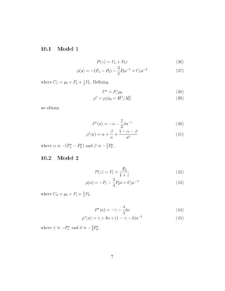
8. 10.3 Hubble function
H
H0
= Ω1 + Ω2 + Ωm (46)
• Model 1
Ω1 = α
Ω2 = β/a
Ωm = Ωm0a−3
Ωm0 = 1 − α − β
• Model 2
Ω1 = γ
Ω2 = δa
Ωm = Ωm0a−3
Ωm0 = 1 − γ − δ
11 G-corrected Holographic Dark Energy [19]
Related to Brans-Dicke gravity
H2
=
8πG(t)
3
(ρm + ρd) + H
˙G
G
(47)
H2
(1 − αG) = H2
0 Ωm0a−3
+ Ωd0a−3(1+ωd)
(48)
where
• ωd = −1
3
− 2
√
Ωd
3c
+ 1
3
αG
• Ωm + Ωd = 1 − αG
• αG = G
G
, and G = dG
d(ln a)
• αG = 0 −→ G(t) = G0
8

9. 12 Exact solutions for Brans-Dicke Cosmol-
ogy with decaying vacuum density [20]
12.1 ˙q = 0 case
H(z) = H0(1 + z)(1+q)
(49)
12.2 ˙q = 0 case
H
H0
=
√
12 − 1 − q0 (z + 1)−
√
12
+
√
12 + 1 + q0
2
48 (z + 1)−
√
12
(50)
9

10. Table 1: Free parameters of each comological model
Model free parameters section
Flat ΛCDM Ωm,0 1.1
Flat Λ(t)CDM Ωm,0 3
Flat DPG Ωrc 5.2
Flat Standard Chaplygin gas A 7.4
Λ(t) Brans-Dicke ˙q = 0 q 12.1
Λ(t) Brans-Dicke ˙q = 0 q0 12.2
ΛCDM Ωm,0, Ωk,0 1.2
Flat ω-CDM Ωm,0, ω 1.3
Kinematics description q0, j0 4
DPG Ωk,0, Ωrc 5.1
Flat Generalized Chaplygin gas A, α 7.2
Standard Chaplygin gas Ωk,0, A 7.3
Parametrized pressure 1 α, β 10.1
Parametrized pressure 2 γ, δ 10.2
ω-CDM Ωm,0, Ωk,0, ω 1.4
Flat CLP-CDM Ωm,0, ω0, ωa 2.1
w parametrization Ωm,0, ω0, ω1 2.2 (eq. 12)
Phantom epoch transition Ωm,0, ω0, z0 2.3 (eq. 14-15)
polytropic Cardassian expansion Ωm,0, q, n 6.2
Generalized Chaplygin gas Ωk,0, A, α 7.1
LTBg Ωin, Ωout, r0 8.1
LTBs Ωin, Ωout, r0 8.2
(1 + z)6
modification / Brane Ωm,0, Ωloops, Ωk,0 9
Bouncing / Brane Ωm,0, Ωloops, Ωk,0 9.1
G-corrected HDE Ωm,0, αG, c 11
w parametrization Ωm,0, ω0, ωa, b 2.2 (eq. 9)
w parametrization Ωm,0, ω0, ωa, ω3 2.2 (eq. 10)
w parametrization Ωm,0, ω0, ωa, ωe 2.2 (eq. 11)
w parametrization Ωm,0, ω0, ω1, ω2 2.2 (eq. 12)
References
[1] Tamara M. Davis, E. Mortsell, J. Sollerman, A.C. Becker, S. Blondin,
et al. Scrutinizing exotic cosmological models using essence supernova
data combined with other cosmological probes. Astrophys.J., 666:716–
10

11. 725, 2007.
[2] Michel Chevallier and David Polarski. Accelerating universes with scal-
ing dark matter. Int.J.Mod.Phys., D10:213–224, 2001.
[3] Eric V. Linder. Exploring the expansion history of the universe.
Phys.Rev.Lett., 90:091301, 2003.
[4] Eric V. Linder and Dragan Huterer. How many dark energy parameters?
Phys.Rev., D72:043509, 2005.
[5] Iker Leanizbarrutia and Diego Sez-Gmez. Parametrizing the transi-
tion to the phantom epoch with Supernovae Ia and Standard Rulers.
Phys.Rev., D90(6):063508, 2014.
[6] H. A. Borges and S. Carneiro. Friedmann cosmology with decaying
vacuum density. Gen. Rel. Grav., 37:1385–1394, 2005.
[7] S. Carneiro, C. Pigozzo, H. A. Borges, and J. S. Alcaniz. Supernova
constraints on decaying vacuum cosmology. Phys. Rev., D74:023532,
2006.
[8] S. Carneiro, M. A. Dantas, C. Pigozzo, and J. S. Alcaniz. Observational
constraints on late-time Λ(t)cosmology.Phys.Rev., D77 : 083504, 2008.
[9] C. Pigozzo, M. A. Dantas, S. Carneiro, and J. S. Alcaniz. Background
tests for L(t)CDM cosmology. arXiv: astro-ph/1007.5290, 2010.
[10] G.R. Dvali, G. Gabadadze, and M. Porrati. Metastable gravitons and
infinite volume extra dimensions. Phys.Lett., B484:112–118, 2000.
[11] Katherine Freese and Matthew Lewis. Cardassian expansion: A Model
in which the universe is flat, matter dominated, and accelerating.
Phys.Lett., B540:1–8, 2002.
[12] Alexander Yu. Kamenshchik, Ugo Moschella, and Vincent Pasquier. An
Alternative to quintessence. Phys.Lett., B511:265–268, 2001.
[13] S. Carneiro and H.A. Borges. On dark degeneracy and interacting mod-
els. JCAP, 1406:010, 2014.
11

12. [14] S. Carneiro and C. Pigozzo. Observational tests of non-adiabatic Chap-
lygin gas. JCAP, 1410:060, 2014.
[15] K. Liao, Y. Pan, and Z.-H. Zhu. Observational constraints on the new
generalized Chaplygin gas model. Research in Astronomy and Astro-
physics, 13:159–169, February 2013.
[16] J. Sollerman, E. M¨ortsell, T. M. Davis, M. Blomqvist, B. Bassett, A. C.
Becker, D. Cinabro, A. V. Filippenko, R. J. Foley, J. Frieman, P. Gar-
navich, H. Lampeitl, J. Marriner, R. Miquel, R. C. Nichol, M. W. Rich-
mond, M. Sako, D. P. Schneider, M. Smith, J. T. Vanderplas, and J. C.
Wheeler. First-year sloan digital sky survey-ii (sdss-ii) supernova results:
Constraints on nonstandard cosmological models. , 703:1374–1385, Oc-
tober 2009.
[17] Marek Szydlowski, Wlodzimierz Godlowski, and Tomasz Stachowiak.
Testing and selection of cosmological models with (1+z)6 corrections.
Phys.Rev., D77:043530, 2008.
[18] Qiang Zhang, Guang Yang, Keji Shen, and Xinhe Meng. Exploring the
universe: two parametric models for the total pressure at low redshift.
2015.
[19] Hamzeh Alavirad and Mohammad Malekjani. Observational constraints
on G-corrected holographic dark energy using a Markov chain Monte
Carlo method. Astrophys.Space Sci., 349:967–974, 2014.
[20] A. E. Montenegro, Jr. and S. Carneiro. Exact solutions of Brans-Dicke
cosmology with decaying vacuum density. Class. Quant. Grav., 24:313–
327, 2007.
12