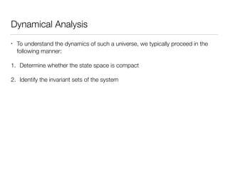
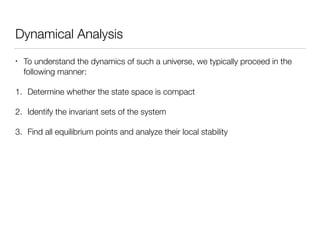
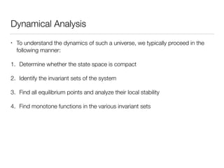
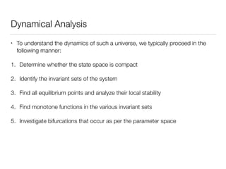
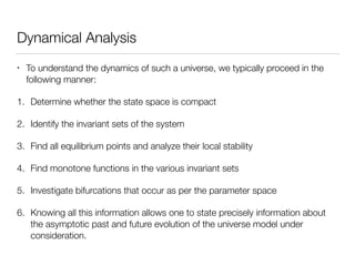
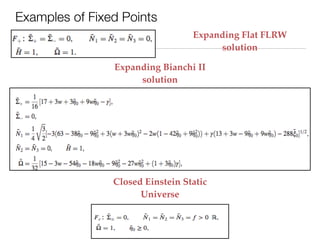
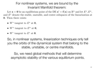
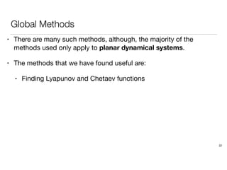
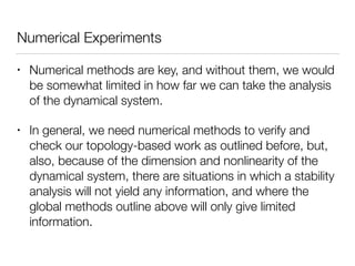
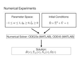
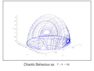
The document discusses applying dynamical systems methods to develop models of the early universe. Specifically, it discusses: 1. Applying these methods to the Einstein field equations to obtain cosmological models that are spatially homogeneous but anisotropic. 2. Describing the process of analyzing the dynamics of these models, which involves identifying invariant sets, equilibrium points, monotone functions, and bifurcations in the parameter space. 3. The importance of numerical methods in understanding the global behavior of these systems, since analytical methods are often limited to local analysis near equilibrium points.

1. Dynamical Systems Methods in
Early-Universe Cosmology
!
SONAD 2014 Talk - May 15, 2014
Ikjyot Singh Kohli, Ph.D. Candidate - Dept.
of Physics and Astronomy - York
University
www.yorku.ca/kohli

2. Introduction

3. Introduction
• Much of my research (with Michael Haslam) is focused on applying
dynamical systems methods to the Einstein field equations to develop
models of the early universe.

4. Introduction
• Much of my research (with Michael Haslam) is focused on applying
dynamical systems methods to the Einstein field equations to develop
models of the early universe.
• Our present-day universe is isotropic (to a very high degree) and spatially
homogeneous. The universe is then described by the Friedmann-
Lemaitre-Robertson-Walker (FLRW) metric.

5. Introduction
• Much of my research (with Michael Haslam) is focused on applying
dynamical systems methods to the Einstein field equations to develop
models of the early universe.
• Our present-day universe is isotropic (to a very high degree) and spatially
homogeneous. The universe is then described by the Friedmann-
Lemaitre-Robertson-Walker (FLRW) metric.
• We would like to understand how this is possible given that the early
universe had a very high temperature and hence was unstable.

6. Introduction
• Much of my research (with Michael Haslam) is focused on applying
dynamical systems methods to the Einstein field equations to develop
models of the early universe.
• Our present-day universe is isotropic (to a very high degree) and spatially
homogeneous. The universe is then described by the Friedmann-
Lemaitre-Robertson-Walker (FLRW) metric.
• We would like to understand how this is possible given that the early
universe had a very high temperature and hence was unstable.
• In our work, we relax the condition of isotropy to obtain cosmological
models that admit Killing vectors that describe spatial translations only,
and as a result are spatially homogeneous and anisotropic in general.
Such models are known as the Bianchi models.

9. Introduction

10. Introduction
• This task is non-trivial, as in General Relativity, space and
time are one entity, spacetime, so it is not immediately
clear how one should essentially “define” a time variable to
get some idea of dynamics.

11. Introduction
• This task is non-trivial, as in General Relativity, space and
time are one entity, spacetime, so it is not immediately
clear how one should essentially “define” a time variable to
get some idea of dynamics.
• I will describe in this talk the method of orthonormal
frames (Ellis and MacCallum, Comm. Math. Phys, 12,
108-141,1969), which turn the Einstein field equations into
a coupled system of nonlinear ordinary differential
equations, and then describe the importance of numerical
methods in understanding the global behaviour of the
system.

12. Spacetime Splitting

13. Spacetime Splitting
• M is a manifold if for every point of M there is an open
neighbourhood of that point for which there is a
continuous one-to-one and onto map f to an open
neighbourhood of R^n for some integer n.

14. Spacetime Splitting
• M is a manifold if for every point of M there is an open
neighbourhood of that point for which there is a
continuous one-to-one and onto map f to an open
neighbourhood of R^n for some integer n.
• The local region of M then can be made to look like R^n
locally.

15. Spacetime Splitting
• M is a manifold if for every point of M there is an open
neighbourhood of that point for which there is a
continuous one-to-one and onto map f to an open
neighbourhood of R^n for some integer n.
• The local region of M then can be made to look like R^n
locally.
• In general relativity, n = 4, for three spatial coordinates,
and one time coordinate.

16. Depiction of a manifold

17. Spacetime Splitting
General Relativity is described by the Einstein field
equations:
Rab
1
2
gabR + gab = kTab
Rab : Ricci tensor
gab : Metric tensor
: Cosmological constant
Tab : Energy-momentum tensor
These are 10 hyperbolic, nonlinear, coupled PDEs!

18. Spacetime Splitting
The solution of these equations is the metric tensor,
typically written in the form:
ds2
= gabdxa
dxb
One sees though, that the EFEs are not your “typical”
field equations, in the sense that the solution is a
metric tensor, and not a time-varying field, as would
be the case with Maxwell’s equations, Navier-Stokes,
etc…

19. Spacetime Splitting
To get a dynamical interpretation, then, we must split our
spacetime into space and time. We accomplish this by
foliating M into a collection of spacelike hypersurfaces and
allow a timelike vector to thread through them.
na
t1
t2
t3
t4

20. (Baumgarte, Shapiro, 2010)
Elliptic
PDEs
Hyperbolic
PDEs

21. Energy-Momentum Tensor
The energy-momentum tensor is given by:
Tab = (µ + p) uaub + gabp 3⇠Hhab 2⌘ ab,
where µ, p, and ab denote the fluid’s energy density, pressure, and shear
respectively, while and denote the bulk and shear viscosity coe cients of
the fluid. Throughout this work, both coe cients are taken to be nonnegative
constants. H denotes the Hubble parameter, and hab uaub + gab is the
standard projection tensor corresponding to the metric signature ( , +, +, +).
See: (Kohli and Haslam, Phys. Rev. D. 87, 063006 (2013)
arXiv: 1207.6132) for further details.
In principle, other terms too, involving heat conduction, but
these are acausal, (parabolic and elliptic PDEs do not
occur in the real, physical universe, except in the sense of
spacetime symmetries).

22. Evolution and Constraint Equations
We will choose an orthonormal frame: {n, e }
That is, n is tangent to a hypersurface-orthogonal
congruence of geodesics, and we obtain:
˙H = H2 2
3
2
µ
1
6
+
1
2
w , (1)
˙ab = 3H ab + 2 uv
(a b)u v Sab 2 ab, (2)
µ = 3H2 2
+
1
2
R, (3)
0 = 3 u
a au
uv
a
b
unbv, (4)
The Einstein field equations:

23. where Sab and R are the three-dimensional spatial curvature and Ricci scalar
and are defined as:
Sab = bab
1
3
bu
u ab 2 uv
(a nb)uav, (1)
R =
1
2
bu
u 6auau
, (2)
where bab = 2nu
anub (nu
u) nab. We have also denoted by v the angular velocity
of the spatial frame.
Using the Jacobi identities, one obtains evolution equations for these vari-
ables as well:
˙nab = Hnab + 2 u
(anb)u + 2 uv
(a nb)u v, (1)
˙aa = Haa
b
aab + uv
a au v, (2)
0 = nb
aab. (3)
The contracted Bianchi identities give the evolution equation for µ as
˙µ = 3H (µ + p) b
a
a
b + 2aaqa
. (4)

24. In addition, we define a dimensionless “time” variable:
dt
d˜⌧
=
1
D
In our research, we are particularly interested in a closed
universe, that is, of topology S^3.
!
The EFEs for such a universe take the form: (Kohli and
Haslam, Phys. Rev. D. 89, 043518 (2014), arXiv:
1311.0389)

25. ˜H0
= (1 ˜H2
)˜q,
˜⌃0
+ = ˜⌃+
˜H ( 2 + ˜q) 6˜⌃+ ˜⌘0
˜S+,
˜⌃0
= ˜⌃ ˜H ( 2 + ˜q) 6˜⌃ ˜⌘0
˜S ,
˜N0
1 = ˜N1
⇣
˜H ˜q 4˜⌃+
⌘
,
˜N0
2 = ˜N2
⇣
˜H ˜q + 2˜⌃+ + 2
p
3˜⌃
⌘
,
˜N0
3 = ˜N3
⇣
˜H ˜q + 2˜⌃+ 2
p
3˜⌃
⌘
,
˜⌦0
= ˜⌦ ˜H ( 1 + 2˜q 3w) + 9 ˜H2 ˜⇠0 + 12˜⌘0
⇣
˜⌃2
+ + ˜⌃2
⌘
where ˜q = 2
⇣
˜⌃2
+ + ˜⌃2
⌘
+
1
2
˜⌦ (1 + 3w)
9
2
˜⇠0
˜H
˜⌦ + ˆ⌃2
+ ˜V = 1
This is a constraint on the initial
conditions

26. Note that:
˜V =
1
12

˜N2
1 + ˜N2
2 + ˜N2
3 2 ˜N1
˜N2 2 ˜N2
˜N3 2 ˜N3
˜N1 + 3
⇣
˜N1
˜N2
˜N3
⌘2/3
˜S+ =
1
6
⇣
˜N2
˜N3
⌘2
˜N1
⇣
2 ˜N1
˜N2
˜N3
⌘
,
˜S =
1
2
p
3
h⇣
˜N3
˜N2
⌘ ⇣
˜N1
˜N2
˜N3
⌘i
.

27. Dynamical Analysis

28. Dynamical Analysis
• To understand the dynamics of such a universe, we typically proceed in the
following manner:

29. Dynamical Analysis
• To understand the dynamics of such a universe, we typically proceed in the
following manner:
1. Determine whether the state space is compact

30. Dynamical Analysis
• To understand the dynamics of such a universe, we typically proceed in the
following manner:
1. Determine whether the state space is compact
2. Identify the invariant sets of the system

31. Dynamical Analysis
• To understand the dynamics of such a universe, we typically proceed in the
following manner:
1. Determine whether the state space is compact
2. Identify the invariant sets of the system
3. Find all equilibrium points and analyze their local stability

32. Dynamical Analysis
• To understand the dynamics of such a universe, we typically proceed in the
following manner:
1. Determine whether the state space is compact
2. Identify the invariant sets of the system
3. Find all equilibrium points and analyze their local stability
4. Find monotone functions in the various invariant sets

33. Dynamical Analysis
• To understand the dynamics of such a universe, we typically proceed in the
following manner:
1. Determine whether the state space is compact
2. Identify the invariant sets of the system
3. Find all equilibrium points and analyze their local stability
4. Find monotone functions in the various invariant sets
5. Investigate bifurcations that occur as per the parameter space

34. Dynamical Analysis
• To understand the dynamics of such a universe, we typically proceed in the
following manner:
1. Determine whether the state space is compact
2. Identify the invariant sets of the system
3. Find all equilibrium points and analyze their local stability
4. Find monotone functions in the various invariant sets
5. Investigate bifurcations that occur as per the parameter space
6. Knowing all this information allows one to state precisely information about
the asymptotic past and future evolution of the universe model under
consideration.

35. Examples of Fixed Points
Expanding Flat FLRW
solution
Expanding Bianchi II
solution
Closed Einstein Static
Universe

36. Stability AnalysisEquilibrium
Point
EFE Solution Local Sink Local Source Saddle
F+
Expanding
k=0 FLRW
solution
Yes No Yes
F-
Contracting
k=0 FLRW
solution
Yes Yes Yes
P+(II)
Expanding
Bianchi Type II
Solution
No No Yes
P_(II) (new
discovery!)
Contracting
Bianchi Type II
Solution
No No Yes

37. 21
For nonlinear systems, we are bound by the
Invariant Manifold theorem:
Let x = 0 be an equilibrium point of the DE x0
= f(x) on Rn
and let Es
, Eu
,
and Ec
denote the stable, unstable, and centre subspaces of the linearization at
0. Then there exists
• Ws
tangent to Es
at 0,
• Wu
tangent to Eu
at 0,
• Wc
tangent to Ec
at 0.
So, in nonlinear systems, linearization techniques only tell
you the orbits of the dynamical system that belong to the
stable, unstable, or centre manifolds.
So, we need global methods that will determine
asymptotic stability of the various equilibrium points.

38. Global Methods
22

39. Global Methods
• There are many such methods, although, the majority of the
methods used only apply to planar dynamical systems.
22

40. Global Methods
• There are many such methods, although, the majority of the
methods used only apply to planar dynamical systems.
• The methods that we have found useful are:
22

41. Global Methods
• There are many such methods, although, the majority of the
methods used only apply to planar dynamical systems.
• The methods that we have found useful are:
• Finding Lyapunov and Chetaev functions
22

42. Global Methods
• There are many such methods, although, the majority of the
methods used only apply to planar dynamical systems.
• The methods that we have found useful are:
• Finding Lyapunov and Chetaev functions
• LaSalle invariance principle
22

43. Global Methods
• There are many such methods, although, the majority of the
methods used only apply to planar dynamical systems.
• The methods that we have found useful are:
• Finding Lyapunov and Chetaev functions
• LaSalle invariance principle
• Monotonicity Principle
22

44. Global Methods
• There are many such methods, although, the majority of the
methods used only apply to planar dynamical systems.
• The methods that we have found useful are:
• Finding Lyapunov and Chetaev functions
• LaSalle invariance principle
• Monotonicity Principle
• Numerical methods
22

45. Global Methods
• There are many such methods, although, the majority of the
methods used only apply to planar dynamical systems.
• The methods that we have found useful are:
• Finding Lyapunov and Chetaev functions
• LaSalle invariance principle
• Monotonicity Principle
• Numerical methods
• The first three give information on the alpha and omega limit sets of
the dynamical system.
22

46. Numerical Experiments

47. Numerical Experiments
• Numerical methods are key, and without them, we would
be somewhat limited in how far we can take the analysis
of the dynamical system.

48. Numerical Experiments
• Numerical methods are key, and without them, we would
be somewhat limited in how far we can take the analysis
of the dynamical system.
• In general, we need numerical methods to verify and
check our topology-based work as outlined before, but,
also, because of the dimension and nonlinearity of the
dynamical system, there are situations in which a stability
analysis will not yield any information, and where the
global methods outline above will only give limited
information.

49. Numerical Experiments
Parameter Space: Initial Conditions:
˜⌦ + ˆ⌃2
+ ˜V = 1
Numerical Solver: ODE23s (MATLAB), ODE45 (MATLAB)
Solution:
˜H( ), ˜±( ), ˜N ( ), ˜( )
1 w 1, ˜0 0, ˜0 0

50. −1
−0.5
0
0.5
1
−1
−0.8
−0.6
−0.4
−0.2
0
0.2
0.4
0.6
0.8
1
0
0.5
1
1.5
2
2.5
3
˜Σ +
˜Σ −
˜N1
Chaotic Behaviour as

53. −1.5
−1
−0.5
0
0.5
1
1.5
−1
−0.5
0
0.5
1
1.5
−1.5
−1
−0.5
0
0.5
1
1.5
˜H
˜Σ +
˜Σ−
This figure shows the dynamical system behavior for ˜0 = 0, ˜0 = 0, and
w = 1/3. In particular, it displays the heteroclinic orbits joining K+ to K ,
where K+ is located at ˜H = 1, and K is located at ˜H = 1 in the figure.
Numerical solutions were computed for 1000 1000. For clarity, we have
displayed solutions for shorter timescales.

54. −0.5
−0.4
−0.3
−0.2
−0.1
0
0.1
0.2
0.3
0.4
0.5
−0.4
−0.3
−0.2
−0.1
0
0.1
0.2
0.3
0.4
0.5
0
0.1
0.2
0.3
0.4
0.5
0.6
0.7
0.8
˜Σ +
˜Σ −
˜N1
This figure shows the dynamical system behaviour for ˜0 = 0, ˜0 = 1/2,
and w = 1/3. The plus sign denotes the equilibrium point F+. The model
also isotropizes as can be seen from the last figure, where ˜± 0 as .
Numerical solutions were computed for 0 1000. For clarity, we have
displayed solutions for shorter timescales.

55. −0.4
−0.3
−0.2
−0.1
0
0.1
0.2
0.3
0.4
0.5
−0.5
−0.4
−0.3
−0.2
−0.1
0
0.1
0.2
0.3
0.4
0.5
−0.5
0
0.5
1
1.5
2
2.5
3
˜Σ +
˜Σ −
˜N1
These figures show the dynamical system behavior for ˜0 = 0, ˜0 = 1/3,
and w = 1. The plus sign denotes the equilibrium point F . The model also
isotropizes as can be seen from the last figure, where ˜± 0 as .
Numerical solutions were computed for 0 1000. For clarity, we have
displayed solutions for shorter timescales.

56. 0 1 2 3 4 5 6 7 8 9 10
−0.5
−0.4
−0.3
−0.2
−0.1
0
0.1
0.2
0.3
0.4
0.5
˜Σ +
˜Σ −

58. • The flat FLRW solution is clearly of primary importance with
respect to modelling the present-day universe, which is
observed to be very close to flat. There are conditions in the
parameter space for which this solution represents a saddle and
a sink.

59. • The flat FLRW solution is clearly of primary importance with
respect to modelling the present-day universe, which is
observed to be very close to flat. There are conditions in the
parameter space for which this solution represents a saddle and
a sink.
• When it is a saddle, the equilibrium point attracts along its stable
manifold and repels along its unstable manifold. Therefore, some
orbits will have an initial attraction to this point, but will eventually
be repelled by it.

60. • The flat FLRW solution is clearly of primary importance with
respect to modelling the present-day universe, which is
observed to be very close to flat. There are conditions in the
parameter space for which this solution represents a saddle and
a sink.
• When it is a saddle, the equilibrium point attracts along its stable
manifold and repels along its unstable manifold. Therefore, some
orbits will have an initial attraction to this point, but will eventually
be repelled by it.
• In the case when it was found to be a sink, all orbits approach
the equilibrium point in the future. Therefore, there exists a time
period and two separate configurations for which our
cosmological model will isotropize and be compatible with
present-day observations of a high degree of isotropy in the
cosmic microwave background.