Download to read offline
![Four Dimensional General Relativity Reduced As ( 1 + 1 ) Gravity
Roa, Ferdinand J. P.
I. Introduction
On its theoretical foundations, General
Relativity is a metric theory of gravity. In place
of Newtonian gravitational potential, the
components of the metric tensor are given
dynamical attributes that are governed by the
metric tensor’s own field equations- Einstein’s
Field Equations. These field equations are
derivable from Einstein-Hilbert action in which
the free Lagrangian (in the absence of interacting
matter terms and cosmological constant) simply
contains the curvature scalar.
By resorting to Kaluza-Klein type of
dimensional reduction, the originally 4D form (
or in originally higher dimensions) of Einstein-
Hilbert action, containing no other terms aside
from the curvature scalar, can be reduced as a 2D
gravity coupled to a scalar field or what is known
as the Einstein-Scalar system.
Two-D models of gravity have become
fashionable previously as toy models used to
study Hawking radiation along with its
associated problems of metric back-reaction and
information loss. The Callan-Giddings-Harvey-
Strominger (CGHS) model has been proposed to
deal with the cited problems. This model as a 2D
gravity is a renormalizable theory of quantum
gravity.
On the related problem of quantization
of gravity that is, reconciling General Relativity
with the postulates of Quantum Mechanics, there
was a consideration pointed out by ‘tHooft that
at a Planckian scale our world is not 3+1
dimensional. Rather, the observable degrees of
freedom can best be described as if they were
Boolean variables defined on a two-dimensional
lattice, evolving with time.
II. 4D General Relativity As A ( 1 + 1 )
Gravity
We start from Einstein-Hilbert action in
four dimensions
Rgxd
~~4
, (1)
then obtain from this an effective action for a ( 1
+ 1 ) gravity upon consideration of the following
fundamental metric form
)sin(
~ 22222
ddedxdxgSd ji
ij
(2)
where ),( 10
xxgij can be thought of as the
components of ( 1 + 1 ) dimensional metric and
together with field ),( 10
xx are functions of
the coordinates ),( 10
xx . We can think of
ji
ij dxdxg as the ( 1 + 1 ) dimensional space-
time, summation over i, j is from 0 to 1.
Proceeding from this set up, we obtain
sin~ 2
geg with g being the
determinant of the lower dimensional metric.
The scalar curvature R
~
on 4d space-time can be
expressed as
22)2(
2))((2
~
eRR L
L
)(2 22
ee L
L
. (3)
We can ignore the last major term in (3)
involving a covariant divergence so that we can
write the effective action as
)2(24
)( RegxdS effEH
sin2))((2 22
eL
L . (4)
This effective action, integration over a
differential four-volume, contains the ( 1 + 1 )
gravity as we take note that all the fields
],[ ijg involved are now solely functions of
the remaining (lower dimensional) coordinates
),( 10
xx . The equations of motion we get from
this action are classically solved for with these
coordinates on a ( 1 + 1 )-space-time.
Equation of Motion for the metric
The effective variation
0
)(
eff
ji
EH
g
S
,
which is equated to zero (by variational
principles) yields the field equations for the
metric
)2(2)2()2(
2
1
jijiji TegRR
. (5)
We choose to work in gauge coordinates](https://image.slidesharecdn.com/dimen-200121103100/85/Dimen-1-320.jpg)
![Four Dimensional General Relativity Reduced As ( 1 + 1 ) Gravity
Roa, Ferdinand J. P.
I. Introduction
On its theoretical foundations, General
Relativity is a metric theory of gravity. In place
of Newtonian gravitational potential, the
components of the metric tensor are given
dynamical attributes that are governed by the
metric tensor’s own field equations- Einstein’s
Field Equations. These field equations are
derivable from Einstein-Hilbert action in which
the free Lagrangian (in the absence of interacting
matter terms and cosmological constant) simply
contains the curvature scalar.
By resorting to Kaluza-Klein type of
dimensional reduction, the originally 4D form (
or in originally higher dimensions) of Einstein-
Hilbert action, containing no other terms aside
from the curvature scalar, can be reduced as a 2D
gravity coupled to a scalar field or what is known
as the Einstein-Scalar system.
Two-D models of gravity have become
fashionable previously as toy models used to
study Hawking radiation along with its
associated problems of metric back-reaction and
information loss. The Callan-Giddings-Harvey-
Strominger (CGHS) model has been proposed to
deal with the cited problems. This model as a 2D
gravity is a renormalizable theory of quantum
gravity.
On the related problem of quantization
of gravity that is, reconciling General Relativity
with the postulates of Quantum Mechanics, there
was a consideration pointed out by ‘tHooft that
at a Planckian scale our world is not 3+1
dimensional. Rather, the observable degrees of
freedom can best be described as if they were
Boolean variables defined on a two-dimensional
lattice, evolving with time.
II. 4D General Relativity As A ( 1 + 1 )
Gravity
We start from Einstein-Hilbert action in
four dimensions
Rgxd
~~4
, (1)
then obtain from this an effective action for a ( 1
+ 1 ) gravity upon consideration of the following
fundamental metric form
)sin(
~ 22222
ddedxdxgSd ji
ij
(2)
where ),( 10
xxgij can be thought of as the
components of ( 1 + 1 ) dimensional metric and
together with field ),( 10
xx are functions of
the coordinates ),( 10
xx . We can think of
ji
ij dxdxg as the ( 1 + 1 ) dimensional space-
time, summation over i, j is from 0 to 1.
Proceeding from this set up, we obtain
sin~ 2
geg with g being the
determinant of the lower dimensional metric.
The scalar curvature R
~
on 4d space-time can be
expressed as
22)2(
2))((2
~
eRR L
L
)(2 22
ee L
L
. (3)
We can ignore the last major term in (3)
involving a covariant divergence so that we can
write the effective action as
)2(24
)( RegxdS effEH
sin2))((2 22
eL
L . (4)
This effective action, integration over a
differential four-volume, contains the ( 1 + 1 )
gravity as we take note that all the fields
],[ ijg involved are now solely functions of
the remaining (lower dimensional) coordinates
),( 10
xx . The equations of motion we get from
this action are classically solved for with these
coordinates on a ( 1 + 1 )-space-time.
Equation of Motion for the metric
The effective variation
0
)(
eff
ji
EH
g
S
,
which is equated to zero (by variational
principles) yields the field equations for the
metric
)2(2)2()2(
2
1
jijiji TegRR
. (5)
We choose to work in gauge coordinates](https://image.slidesharecdn.com/dimen-200121103100/75/Dimen-1-2048.jpg)

Note that in this solution rx 1
but
1
x is
related to r by
)exp(1)exp( 1
rcrcxc FFF (11)
for which the effective curvature in )(effEHS is
twice the curvature on 2-sphere
22
)( /44
~
reR eff
. (12)
For later purposes we should also write the
relations of the gauge coordinates to r and
0
x ,
given (11):
)](exp[1)exp( 0
rxcrcxc FFF
,
(13a)
)](exp[1)exp( 0
rxcrcxc FFF
(13b)
III. Causal Structure of the ( 1 + 1 )
Space-time
As thought of,
ji
ij dxdxg is the ( 1 + 1
) dimensional space-time,
dxdx
rc
dxdxg
F
ji
ij
1
1 . (14)
We can notice then that (11) can cover
only the region at and (or) above the critical
value of r, 1rcF . That is, relation (11) is for
the region where
rcF
1
0 ,
0
x ,
x and
x .
To cover the region where r is below
1
Fc , we can switch sign in the originally time-
like ( 1 + 1 ) space-time (14) to become space-
like. Thus, in this region ( 10 rcF ), the (
) metric component is
2/)1/1(2/2
rceg F
as a
consequence of the new relations
)exp()1()exp( 1
rcrcxc FFF , (15a)
)](exp[1)exp( 0
rxcrcxc FFF
(15b)
and
)](exp[1)exp( 0
rxcrcxc FFF
(15c)
that can cover the region 10 rcF .
In both these regions, constraints (7a to
7c) and equation (8) still hold. That is, the
physics of both regions is still described by the
same set of equations.](https://image.slidesharecdn.com/dimen-200121103100/85/Dimen-2-320.jpg)
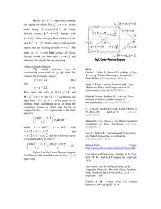


This document summarizes the dimensional reduction of 4D general relativity to a (1+1) gravity model. It shows that the Einstein-Hilbert action in 4D can be reduced to an effective action for a (1+1) gravity coupled to a scalar field. The equations of motion for the reduced metric and scalar field are derived. The causal structure of the resulting (1+1)-dimensional spacetime is examined, with the regions above and below a critical radius value related by a change of coordinates. A Carter-Penrose diagram illustrates the causal structure.


![Polymer [ बहुलक ] Chemistry Notes PDF - Irfanullah Mehar - JJ Sir Chemistry.pdf](https://cdn.slidesharecdn.com/ss_thumbnails/polymerchemistrynotespdf-irfanullahmehar-jjsirchemistry-260210172118-3f9b37f7-thumbnail.jpg?width=640&height=640&fit=bounds)


