Digital Implementation of Artificial Neural Network for Function Approximation and Pressure Control Applications

IOSR Journal of Electronics and Communication Engineering (IOSR-JECE)
e-ISSN: 2278-2834,p- ISSN: 2278-8735.Volume 5, Issue 5 (Mar. - Apr. 2013), PP 34-39
www.iosrjournals.org
www.iosrjournals.org 34 | Page
Digital Implementation of Artificial Neural Network for Function
Approximation and Pressure Control Applications
Sangeetha T#1
, Meenal C#2
1,2
Department of Electronics and Communication Engineering
1
PG Scholar, Mount Zion College of Engineering and Technology, Pudukkottai, Tamil Nadu, India.
2
Assistant Professor, Mount Zion College of Engineering & Technology, Pudukkottai, TamilNadu India
Abstract: The soft computing algorithms are being nowadays used for various multi input multi output
complicated non linear control applications. This paper presented the development and implementation of back
propagation of multilayer perceptron architecture developed in FPGA using VHDL. The usage of the FPGA
(Field Programmable Gate Array) for neural network implementation provides flexibility in programmable
systems. For the neural network based instrument prototype in real time application. The conventional specific
VLSI neural chip design suffers the limitation in time and cost. With low precision artificial neural network
design, FPGA have higher speed and smaller size for real time application than the VLSI design. The
challenges are finding an architecture that minimizes the hardware cost, maximizing the performance,
accuracy. The goal of this work is to realize the hardware implementation of neural network using FPGA.
Digital system architecture is presented using Very High Speed Integrated Circuits Hardware Description
Language (VHDL)and is implemented in FPGA chip. MATLAB ANN programming and tools are used for
training the ANN. The trained weights are stored in different RAM, and is implemented in FPGA. The design
was tested on a FPGA demo board.
Keywords- Backpropagation, field programmable gate array (FPGA) hardware implementation, multilayer
perceptron, pressure sensor, Xilinx FPGA.
I. Introduction
Implementation of ANNs falls into two categories: Software implementation and hardware
implementation. ANNs are implemented in software, and are trained and simulated on general-purpose
sequential computers for emulating a wide range of neural networks models. Software implementations offer
flexibility. However hardware implementations are essential for applicability and for taking the advantage of
ANN’s inherent parallelism. Specific-purpose fixed hardware implementations(i.e. VLSI) are dedicated to a
specific ANN model. VLSI implementations of ANNs provide high speed in real time applications and
compactness. However, they lackflexibility for structural modification and are prohibitively costly.
Software implementations can be quickly constructed, adapted, and tested for a wide range of
applications. However, in some cases, the use of hardware architectures matching the parallel structure of ANNs
is desirable to optimize performance or reduce the cost of the implementation, particularly for applications
demanding high performance. Unfortunately, hardware platforms suffer from several unique disadvantages such
as difficulties in achieving high data precision with relation to hardware cost, the high hardware cost of the
necessary calculations, and the inflexibility of the platform as compared to software.
In this work, aimed address some of these disadvantages by developing and implementing a field
programmable gate array (FPGA)-based architecture of a neural network with learning capability. Exploiting
the reconfigurability of FPGAs, we are able to perform fast prototyping of hardware-based ANNs to find
optimal application specific configurations. In particular, the ability to quickly generate a range of hardware
configurations gives us the ability to perform a rapid design space exploration navigating the cost/speed/accu-
racy tradeoffs affecting hardware-based ANNs.
II. ARTIFICIAL NEURAL NETWORKS (Anns)
Artificial neural networks (ANN’s, or simply NN’s) are inspired by biological nervous systems and
consist of simple processing elements (PE, artificial neurons) that are interconnected by weighted connections.
The predominantly used structure is a multilayered feed-forward network (multilayer perception),i.e., the nodes
(neurons) are arranged in several layers (input layer, hidden layers, output layer), and the information flow is
only between adjacent layers [4].An artificial neuron is a very simple processing unit. It calculates the weighted
sum of its inputs and passes it through a nonlinear transfer function to produce its output signal.The
predominantly used transfer functions are so-called “sigmoid” or “squashing” functions that compress an
infinite input range to a finite output range, e.g., [-1, +1].

Digital Implementation of Artificial Neural Network for Function Approximation and Pressure
Fig.1 processing element Fig.2 Multilayer perception model
Neural networks can be “trained” to solve problems that are difficult to solve by conventional computer
algorithms. Training refers to an adjustment of the connection weights, based on a number of training examples
that consist of specified inputs and corresponding target outputs. Training is an incremental process where after
each presentation of a training example, the weights are adjusted to reduce the discrepancy between the network
and the target output. Popular learning algorithms are variants of gradient descent (e.g., error-backpropagation) ,
radial basis function adjustments [4], etc. Neural networks are well suited to a variety of nonlinear problem
solving tasks. For example, tasks related to the organization, classification, and recognition of large sets of
inputs.
2.1 Multilayer Perceptrons (MLPs)
MLPs (Fig. 2) are layered fully connected feed-forward networks. That is, all PEs (Fig. 1) in two
consecutive layers are connected to one another in the forward direction.
During the network's forward pass each PE computes its outputykfrom the input ik it receives from each PE
in the preceding layer as shown here
yk= )(vkk (1)
where k is the squashing function of PE k whose role is to constrain the value of the local field
vk=   kwkjikj  (2)
Wkj is the weight of the synapse connecting neuron k to neuron j in the previous layer, and k k is the bias of
neuron k. Equation (1) is computed sequentially by layer from the first hidden layer which receives its input
from the input layer to the output layer, producing one output vector corresponding to one input vector.
The network’s behavior is defined by the values of its weights and bias. It follows that in network
training the weights and biases are the subjects of that training. Training is performed using the backpropagation
algorithm after every forward pass of the network.
2.2 Backpropagation Algorithm
The backpropagation learning algorithm allows us to compute the error of a network at the output,
then propagate that error backwards to the hidden layers of the network adjusting the weights of the neurons
responsible for the error. The network uses the error to adjust the weights in an effort to let the output yj
approach the desired output dj.
Backpropagation minimizes the overall network error by calculating an error gradient for each neuron
from which a weight change ∆wjiis computed for each synapse of the neuron. The error gradient is then
recalculated and propagated backwards to the previous layer until weight changes have been calculated for all
layers from the output to the first hidden layer.
The weight correction for a synaptic weight connecting neuron i to neuron j mandated by backpropagation is
defined by the delta rule
∆wji= jyi (3)
where is the learning rate parameter, j is the local gradient of neuron j, and yi is the output of neuron i in the
previous layer.
Calculation of the error gradient can be divided into two cases: for neurons in the output layer and for neurons in
the hidden layers. This is an important distinction because we must be careful to account for the effect that
changing the output of one neuron will have on subsequent neurons. For output neurons, the standard definition
of the local gradient applies
)(' vjjejj   (4)
For neurons in a hidden layer, we must account for the local gradients already computed for neurons in the
following layers up to the output layer. The new term will replace the calculated error e since, because hidden

neurons are not visible from outside of the network, it is impossible to calculate an error for them. So, we add a
term that accounts for the previously calculated local gradients
 kwkjvjjj  )(' (5)
Wherej is the hidden neuron whose new weight we are calculating, and k is an index for each neuron in the next
layer connected to j.
As we can see from (4) and (5), we are rewe are required to differentiate the activation function j with
respect to its own argument, the induced local field vj. In order for this to be possible, the activation function
must of course be differentiable. This means that we cannot use non continuous activation functions in a back-
propagation-based network. Two continuous, nonlinear activation functions commonly used in back
propagation networks are the sigmoid function
)(vj 1∕1+e-avj (6)
Training is performed multiple times over all input vectors in the training set. Weights may be updated
incrementally after each input vector is presented or cumulatively after the training set in its entirety has been
presented (one training epoch). This second approach, called batch learning, is an optimization of the back
propagation algorithm designed to improve convergence by preventing individual input vectors from causing
the computed error gradient to proceed in incorrect direction.
III. Field Programmable Gate Array And Very High Hardware Description Language
FPGAs consist of three basic blocks that are configurable logic blocks, in-out blocks and connection
blocks. Logic blocks perform logic function. Connection blocks connect logic blocks with in-out blocks. These
structures consist of routing channels and programmable switches. Routing process is effectively connection
logic blocks exist different distance the others [6].
FPGAs are chosen for implementation ANNs with the following reason:
 They can be applied a wide range of logic gates starting with tens of thousands up to few millions gates.
 They can be reconfigured to change logic function while resident in the system.
 FPGAs have short design cycle that leads to fairly inexpensive logic design.
 FPGAs have parallelism in their nature. Thus, they have parallel computing environment and allows logic
cycle design to work parallel.
 They have powerful design, programming and syntheses tools.
The architecture of ANNs must be specified with schematic or algorithmic at first step of FPGAs based
system design. When ANNs based FPGAs system design specify the architecture of ANNs from a symbolic
level. This level allows us using VHDL which stands for VHSIC (Very High Speed Integrated Circuit)
Hardware Programming Language [7]. VHDL allows many levels of abstractions, and permits accurate
description of electronic components ranging from simple logic gates to microprocessors. VHDL have tools
needed for description and simulation which leads to a lower production cost.
IV. Hardware Implementation
4.1 system architecture
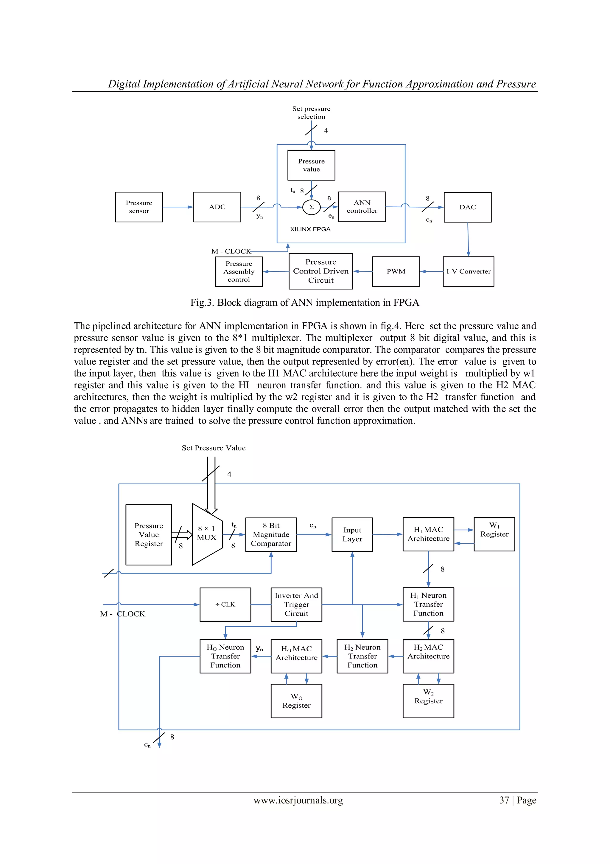
The proposed system architecture is shown in fig.3 The proposed system working principles and
detailed description is given below. The pressure sensor input is in analog nature this analog input is given to
analog to digital converter. The signal conditioning circuit (ADC) convert analog signal into 8 bit digital signal.
This 8 bit digital signal is given to the summing block then set the pressure selection value is given to the
summing block .The summing block act as comparator, the comparator compares the input value and the
reference value and give the difference value and it is denoted by en (error value) . The error value is en is
given to the ANN controller unit here the neural network is designed and trained to using the multilayer
perceptron architecture and the back propagation algorithm. Then compute overall error and the output is given
to digital to analog converter, then the digital to analog converter output is in current form so it is given to the
current to voltage converter. Then the output is given to the modulation block, here pulse width modulation
is done. The modulated signal given to pressure assembly control block. This is compute the overall error and
measure the pressure value and function approximation. The .pressure control driven circuit is used to activate
pressure assembly control block.

ADC
Pressure
value
Pressure
sensor
ANN
controller
DAC
PWM I-V Converter
Pressure
Control Driven
Circuit
Pressure
Assembly
control
Σ
XILINX FPGA
M - CLOCK
88 8
8
4
Set pressure
selection
tn
en
cn
yn
Fig.3. Block diagram of ANN implementation in FPGA
The pipelined architecture for ANN implementation in FPGA is shown in fig.4. Here set the pressure value and
pressure sensor value is given to the 8*1 multiplexer. The multiplexer output 8 bit digital value, and this is
represented by tn. This value is given to the 8 bit magnitude comparator. The comparator compares the pressure
value register and the set pressure value, then the output represented by error(en). The error value is given to
the input layer, then this value is given to the H1 MAC architecture here the input weight is multiplied by w1
register and this value is given to the HI neuron transfer function. and this value is given to the H2 MAC
architectures, then the weight is multiplied by the w2 register and it is given to the H2 transfer function and
the error propagates to hidden layer finally compute the overall error then the output matched with the set the
value . and ANNs are trained to solve the pressure control function approximation.
Pressure
Value
Register
8 Bit
Magnitude
Comparator
Input
Layer
H1 MAC
Architecture
H1 Neuron
Transfer
Function
W1
Register
W2
Register
WO
Register
HO MAC
Architecture
H2 MAC
Architecture
HO Neuron
Transfer
Function
H2 Neuron
Transfer
Function
8 × 1
MUX
8
tn en
÷ CLK
Inverter And
Trigger
Circuit
8
M - CLOCK
ynyn
cn
8
8
8
4
Set Pressure Value

V. Experimental Results
The artificial neural network is designed and implement the pressure control application. The network
implementation built using the MATLAB neural network tool box and find the minimum mean square error.
0 5 10 15 20 25 30
0
5
10
15
20
25
30
Behavior of Unknown System
Pressure(Pa)
ArbitraryOutputVoltage(v)
Fig.5. Behavior of unknown system
0 5 10 15 20 25 30
0
5
10
15
20
25
30
Training data and Testing data
Pressure(Pa)
Fig.6. Training data and testing data
0 5 10 15 20 25 30
-5
0
5
10
15
20
25
30
Original o/p & NN o/p without training
Pressure(Pa)
Fig 7. Original output and NN output without training
0 5 10 15 20 25 30
-5
0
5
10
15
20
25
30
Original o/p & trained NN o/p
Pressure(Pa)
Fig.8 originl output and NN output
Fig.9 Neural network training performance
Fig.10 neural network toolbox
0 5 10 15 20 25 30 35
-0.1
-0.05
0
0.05
0.1
0.15
Error profile
Check data points
Error
Fig.11 Error profile

Fig.12 Simulation Result of Pressure Controller Fig.13 Schematic of Pressure
Controller
VI. Conclusion
In this paper, presented the development and implementation of a pipelined FPGA-based architecture
for feed-forward multilayer perception architecture with back propagation of learning algorithm. In general, it
is shown that implementation of neural networks using FPGAs. The resultant neural networks are modular,
compact, and efficient and the number of neurons, number of hidden layers and number of inputs are easily
changed. However this study shows that FPGAs are versatile devices for implementing many different
applications. The VHDL-FPGA combination is shown to be a very powerful embedded system design tool, with
low cost, reliability. In conclusion, the ANNs are trained and testing the system using the function
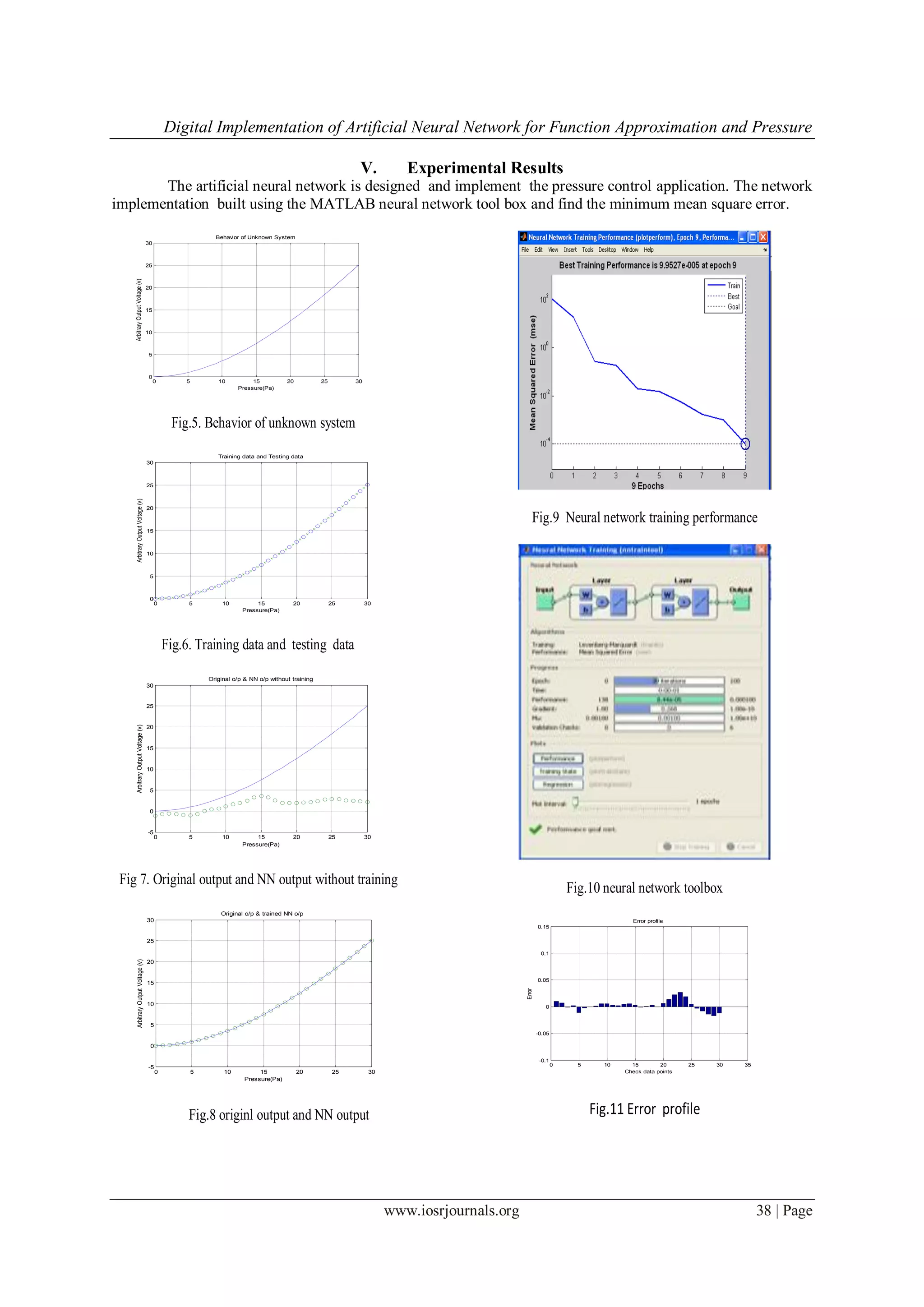
approximation for pressure control application. It showed that the system can reach best training performance
i.e9.957at epoch9 and the minimum mean square error is 10-4
.These best training weights are implemented in
FPGA board.
References
[1] M. Paliwal and U. A. Kumar, “Neural networks and statistical techniques: A review of applications,” Expert Systems With
Applications,vol. 36, pp. 2–17, 2009
[2] R. Gadea, R. C. Palero, J. C. Boluda, and A. S. Cortes, “FPGA implementation of a pipelined on-line back propagation,” J. VLSI
SignalProcess., vol. 40, pp. 189–213, 2005.
[3] A. R. Ormondi and J. Rajapakse, FPGA Implementations of Neural Networks. New York: Springer, 2006
[4] M. Tommiska, “Efficient digital implementation of the sigmoid function for reprogrammable logic,” in Proc. IEE Comput. Digital
Tech., 2003, vol.150, pp. 403–4
[5] E. Sanchez, “FPGA implementation of an adaptable-size neural network,” in Proc. Int. Conf. ANN, 1996, vol. 1112, pp. 383–388
[6] J. Li and D.Liang,“A survey of FPGA-based hardware implementation of ANNs,” in Proc. Int. Conf. Neural Networks Brain,
2005, vol. 2, pp. 915–91
[7] R. Gadea, J. Cerda, F. Ballester, and A. Mocholi, “Artificial neural network implementation on a single FPGA of a pipeline on-line
backpropagation,” in Proc. Int. Symp.Syst. Synthesis, 2000, pp. 225–230
[8] P. Ferreiraa, P. Ribeiroa, A. Antunes, and F. M. Dias, “A high bit resolution FPGA implementation of a FNN with a new algorithm
for the activation function,” Neurocomputing, vol. 71, pp. 71–77, 2007.
[9] S.Tatikonda and P.Agarwal, “Field programmable gate array (FPGA) based neural network implementation of motion control and
fault diagnosis of induction motor drive,” in Proc. IEEE Conf. Ind. Tech., 2008, pp. 1–6.
[10] A. Mellit, H.Mekki, A. Messai, and H. Salhi, “FPGA-based implementation of an intelligent simulator for stand-alone
photovoltaic system,” Expert Systems With Applications, vol. 37, pp. 6036–6051, 2010

Digital Implementation of Artificial Neural Network for Function Approximation and Pressure Control Applications

More Related Content

What's hot

Viewers also liked

Similar to Digital Implementation of Artificial Neural Network for Function Approximation and Pressure Control Applications

More from IOSR Journals

Recently uploaded

Digital Implementation of Artificial Neural Network for Function Approximation and Pressure Control Applications