Control Analysis of a mass- loaded String

International Journal of Innovative Research in Advanced Engineering (IJIRAE) ISSN: 2349-2763
Issue 12, Volume 2 (December 2015) www.ijirae.com
_________________________________________________________________________________________________
IJIRAE: Impact Factor Value - ISRAJIF: 1.857 | PIF: 2.469 | Jour Info: 4.085 | Index Copernicus 2014 = 6.57
© 2014- 15, IJIRAE- All Rights Reserved Page -61
Control Analysis of a mass- loaded String
Giman KIM*
Department of Mechanical System Engineering,
Kumoh National Institute of Technology
Korea
Abstract— This study deals with the active control of the dynamic response of a string with fixed ends and mass
loaded by a point mass. It has been controlled actively by means of a feed forward control method. A point mass of a
string is considered as a vibrating receiver which be forced to vibrate by a vibrating source being positioned on the
string. By analyzing the motion of a string, the equation of motion for a string was derived by using a method of
variation of parameters. To define the optimal conditions of a controller, the cost function, which denotes the dynamic
response at the point mass of a string was evaluated numerically. The possibility of reduction of a dynamic response
was found to depend on the location of a control force, the magnitude of a point mass and a forcing frequency.
Keywords— Active control, a point mass, feed forward control method, a method of variation of parameters, cost
function
I. INTRODUCTION
In the industrial fields, vibration phenomena of machines and structures had been serious problems to be solved for
the green environmental conditions. So far a lot of researches have been performed to analyze and control the vibration
phenomena induced by machining operations in the past decades. Currently the fast manufacturing time and the accurate
level of the machining tools are known to be the important factors of the optimal design condition. In case of the needs of
the high speed operation, the vibration phenomenon should be one of the overcoming troubles for the stability of the
machine structure.
For the simplification of the complex structures, each part of the machines is considered as a continuous system such
as string, beam, plate or shell. Hence, the vibration characteristics of a continuous system had been studied by lots of
persons. Recently for the investigation of the vibration characteristics, the vibration energy flow and the dynamic
response of a beam, plate, shell or some compound system have been analyzed. By using a model of an elastic beam, the
vibration energy and control technologies had been presented [1-3]. Furthermore, the complex frame which is the
assembly of several beams had been used to analyze and control the vibration characteristics [4-5]. The feedforward
control method had been proven to become the convenient control method for the known forcing frequency zone [6-8].
In this study a vibrating system which consists of a point mass and a string with a primary source and a control force is
modelled to analyze and control the dynamic response of a string. The edges conditions of a string are fixed. Based on
the wave equation, the vibration of a string will be discussed. To define the optimal conditions for the control of the
dynamic response, the cost function will be evaluated numerically by using the Mathmatica program of ‘FindMinimum’.
Fig. 1 shows the theoretical model of a uniformly stretched string which is mass-loaded by a point mass and excited to
vibration in the plane.
Fig. 1: Theoretical model
Fp (source), Fc (control force), A point mass (mass (mo)),
STRING PROPERTIES (LENGTH (L), DENSITY (), CONSTANT TENSION (T))
II. THE GOVERNING EQUATION
A uniformly stretched string of mass density  and length L fixed at both ends is subjected to a point mass mo located
at a distance of xo from the left end of the string. The governing equation of a vibrating mass-loaded string can be written
as:
      .
),(),(),(
T 2
2
2
2
2
2
ti
cc
ti
ppoo exxFexxF
t
txu
xxm
t
txu
x
txu 
 







 (1)
Where u(x,t) represent the displacement of a string and  is the circular frequency. In Eq. (1), the source and control
forces are given as the time harmonic forcing function. The displacement (u(x,t)) is expressed into the terms of the time
harmonic motion as,

_________________________________________________________________________________________________
.)(),( ti
exytxu 
 (2)
Where y(x) means the deflection of a string. By inserting Eq. (2) into Eq. (1) and then suppressing the time term, Eq.(1)
can be rearranged as,
     .)()(
)( 2
2
2
2
c
c
p
p
oo
o
xx
T
F
xx
T
F
xxxy
T
m
xyk
x
xy




 (3)
Where the wave number k2
=2
/T. The total solution of Eq. (3) can be expressed into the sum of a homogeneous
solution (yh) and a particular solution (yp) as
).()()( xyxyxy ph  (4)
The homogeneous solution is determined by letting the right side of Eq. (3) be zero and then becomes as
.cossin)( kxBkxAxyh  (5)
Where the constants A and Bcan be obtained by using the boundary conditions of a string. Here the particular solution
can be solved by means of a method of variation of parameters and then be assumed as
.cos)(sin)()( 21 kxxVkxxVxy p  (6)
Where the coefficients V1 and V2 are can be determined by means of the method of variation of parameters and defined as
follows
        .sin
1
)(cos
1
)( 21  dfk
k
xVanddfk
k
xV
xx
 
       .)(,
2
c
c
p
p
oo
o
x
T
F
x
T
F
xxy
T
m
ffunctionforcingthewhere  


The final form of the particular solution can be obtained by using Eqs. (5) and (6). The complete solution of Eq. (3) can
be written as
         
    .sin)(
sinsincossin)(
2
ooo
o
cc
c
pp
p
xxHxxkxy
kT
m
xxHxxk
kT
F
xxHxxk
kT
F
kxBkxAxy



(7)
Where H(x) represents the Heaviside unit step function and the quantity, y(xo) can be evaluated by inserting x=xo into
Eq. (7) and then becomes as
         .sinsincossin)( coco
c
popo
p
ooo xxHxxk
kT
F
xxHxxk
kT
F
kxBkxAxy 
By inserting y(xo) into Eq. (7) and then using the boundary conditions, the final solution of the dynamic response of a
string becomes as,
   
           
           ].sinsin[sin
]sinsin[sin
sinsinsin
2
1
)(
2
2
2
cocooo
o
cc
c
popooo
o
pp
p
ooo
o
xxHxxkxxHxxk
kT
m
xxHxxk
kT
F
xxHxxkxxHxxk
kT
m
xxHxxk
kT
F
xxHxxkkx
kT
m
kx
A
A
xy












(8)
Where the constant functions A1 and A2 are as follows,
       
       
 .sinsinsin2
]sinsin[sin
]sinsin[sin1
2
2
2
oo
o
cocoo
o
c
c
popoo
o
p
p
xLkkx
kT
m
kLA
and
xxHxxkxLk
kT
m
xLk
kT
F
xxHxxkxLk
kT
m
xLk
kT
F
A






Equation (8) is employed as the control factor to be reduced actively by applying the control force to a string. So the cost
function for the reduction of dynamic response of a point mass can be defined as
  .)(Re
2
oxyal (9)
Here the optimal value of the control force which leads to the minimum value of Eq. (9) can be obtained numerically as
the following process,

_________________________________________________________________________________________________
 .optimalcf ffofonMinimizati  (10)
Where the control force is evaluated in terms of the nondimensional form which be based on the source force. As
mentioned before, the optimal values have been obtained by using Mathmatica program -‘FindMinimum’.
III. NUMERICAL RESULTS AND DISCUSSION
All values obtained in this study have been expressed into the nondimensional forms. In Table 1, the nondimensional
properties and the given values are introduced as
TABLE I
NONDIMENSIONAL PROPERTIES AND THE GIVEN VALUES
Expression form Value
A mass ratio m = mo/(mo+L) variable
Source force Fp 1
A structural damping ratio 0.001
A point mass location Xo=xo/L 0.4
Source location Xp=xp/L 0.6
Control force location Xc=xc/L variable
Control force fc=Fc/Fp
A. Resonance Frequency Equation
In Eq. (8), the denominator part A2 vanishes for certain specific values of the wave number k. The roots of
denominator which are expressed in r by k2
=2
/T are called the resonance frequencies for the string. So the resonance
frequency equation becomes as,
  .0sinsinsin)(
2
 oo
o
xLkkx
kT
m
kLkF
 (11)
Here Eq. (11) can be rewritten in terms of the nondimensional form as,
  .01sinsinsin)(  oo XXmF 


 (12)
mand
LmL
T
frequencyensionalnonaWhere
o


 1
)(
)(dim 



Equation (12) is a transcendental equation in  and its roots must be obtained numerically. The first two roots of Eq.
(12) were found numerically. In Fig. 1, the first (1) and the second (2) resonance frequency loci for four different mass
ratios (m=0, 0.1, 0.2, 0.3) are plotted versus the location of the point mass (Xo). As the magnitude of a point mass is
smaller, the less variance be experienced. For the first resonance frequency, as the location of a point mass is close to the
center, the values are getting smaller in comparison with no point mass case. But in case of the second resonance
frequency, the gap between the maximum and minimum values is getting bigger than that of the first resonance
frequency.
Fig. 2 A nondimensional frequency vs. location of a point mass : 1 and 2
0. 0.1 0.2 0.3 0.4 0.5 0.6 0.7 0.8 0.9 1.
4
5
6
7
8


Location of a point mass
0. 0.1 0.2 0.3 0.4 0.5 0.6 0.7 0.8 0.9 1.
1.
1.
2.
2.
3.
3.
4.
4.
5.


Location of a point mass

_________________________________________________________________________________________________
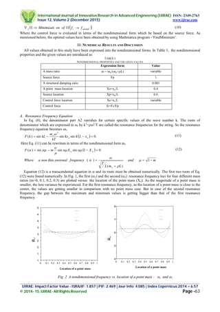
B. Reduction of Dynamic Response of a Point mass
The reduction level of the dynamic response of a point mass is expressed in the value of decibel [dB] as 20Log10[y(xo)].
The optimal control force was evaluated by Eq. (10) with the fixed locations which are the source location (Xp=0.6) and
the point mass location (Xo=0.4). In Fig. 3, (A) and (B) show the variations of control force versus its location for two
cases of nondimensional frequencies (=3, 20), respectively. For the low frequency zone (=3), the regular pattern of
force loci were found for three different mass ratios. As the control force is located closely to the center of string, the
magnitude is getting smaller. However at high frequency zone (=20), the magnitudes of control force are too changable
to be estimated. In Fig. 4, the dynamic responses of a point mass were plotted against nondimensional frequency (). In
case of Fig. 4 (A), the dynamic response of a point mass was controlled only for =3. Hence, the reduction was done
well for the low frequency zone (=1~5). But for the other frequency zone, the given optimal control force is getting
ineffective or worse to reduction level. Similar case is shown in Fig. 4 (B) for =20.
(A) (B)
Fig. 3 Magnitude of Control force vs. location of Control force for three mass ratio : Xp=0.6, Xo=0.4, (A) =3 and (B) =20
(A) (B)
Fig. 4 Dynamic response of a point mass vs. : Xp=0.6, Xo=0.4, (A) =3 and (B) =20
IV.CONCLUSIONS
On the bases of the analyses in this paper, the conclusions are obtained as follows, - Feedforward control method is
proven to give the satisfactory results for the reduction of the dynamic response of a point mass which is forced to vibrate
by the source of the string. In Fig. (5), the reduction values in dB were plotted versus location of Control force for three
nondimensional frequencies All values of reduction are known to be over 300 dB. It is surely noted that the
reduction of dynamic response of a point mass be done successfully up to zero deflection level.
0.0 0.2 0.4 0.6 0.8 1.0
0.0
0.5
1.0
1.5
2.0
2.5
3.0
3.5
4.0
m=0.1
m=0.2
m=0.3
MagnitudeofControlforce
Locationof Control force(fc)
0.0 0.2 0.4 0.6 0.8 1.0
0.0
0.5
1.0
1.5
2.0
2.5
3.0
3.5
4.0
MagnitudeofControlforce
Location of Control force(fc)
m=0.1
m=0.2
m=0.3

_________________________________________________________________________________________________
Fig. 5 Reduction of Dynamic response [dB] vs. Location of Control force: Xp=0.6, Xo=0.4, m=0.2
- The location of the control force is known to become the important factor for the control strategy.
- At the low frequencies, the optimal locations of the control force are known to be positioned close to the center of the
string.
ACKNOWLEDGMENT
This paper was supported by Research Fund, Kumoh National Institute of Technology.
REFERENCES
[1] Pan, J. and Hansen, C. H., “Active control of total vibratory power flow in a beam. I : Physical System Analysis,” J.
Acoust. Soc. Am. vol. 89, No. 1, pp. 200-209, 1991.
[2] Enelund, M, “Mechanical power flow and wave propagation in infinite beams on elastic foundations,” 4th
international congress on intensity techniques, pp. 231-238, 1993.
[3] Schwenk, A. E., Sommerfeldt, S. D. and Hayek, S. I., “Adaptive control of structural intensity associated with
bending waves in a beam,” J. Acoust. Soc. Am. vol. 96, No. 5, pp. 2826-2835, 1994.
[4] Beale, L. S. and Accorsi, M. L, “Power flow in two and three dimensional frame structures,” Journal of Sound and
Vibration, vol. 185, No. 4, pp. 685-702, 1995.
[5] Farag, N. H. and Pan, J. , “Dynamic response and power flow in two-dimensional coupled beam structures under in-
plane loading,” J. Acoust. Soc. Am., vol. 99, No. 5, pp. 2930-2937, 1996.
[6] Nam, M., Hayek, S. I. and Sommerfeldt, S. D., “Active control of structural intensity in connected
structures,” Proceedings of the Conference Active 95, pp. 209-220, 1995.
[7] Kim, G. M., “Active control of vibrational intensity at a reference point in an infinite elastic plate,” Transactions of
the Korean Society for Noise and Vibration Engineering, vol. 11. No. 4, pp. 22-30, 2001.
[8] Kim, G. M. and Choi, S. D., “Active control of dynamic response for a discrete system in an elastic structure,”
Advanced Materials Research, vol.505, pp. 512-516, 2012.
0.0 0.2 0.4 0.6 0.8 1.0
100
150
200
250
300
350
400



ReductionofDynamicResponse[dB]
LocationofControlforce(fc)

Control Analysis of a mass- loaded String

More Related Content

What's hot

Viewers also liked

Similar to Control Analysis of a mass- loaded String

More from AM Publications

Recently uploaded

Control Analysis of a mass- loaded String