Downloaded 18 times


![0
2
1
2
C
m n
= +
+ +
[1 ]wα
α
−
< >
0CEstimation of
For fully developed bubbly flow (Ishii)
0 0 ,
g
l l
GD
C C
ρ
ρ µ
= ÷
Assuming power law profiles for α and j](https://image.slidesharecdn.com/driftflux-160814081619/85/Drift-flux-31-320.jpg)

![For boiling bubbly flow in an internally heated annulus
3.12< >0.212
Co= 1.2 - 0.2 [1 - e ]
g
l
α
ρ
ρ
In downward two-phase flow for all flow regimes
0C =(- 0.0214<j*> + 0.772) + (0.0214<j*> + 0.228) for (-20) <j*> < 0
g
l
ρ
ρ
≤
0.00848[<j*>+20] 0.00848[<j*>+20]
oC =(0.2e +1) - 02e for < j*> < (-20)
g
l
ρ
ρ
÷
÷
Where <j*
> =
2 j
j
u](https://image.slidesharecdn.com/driftflux-160814081619/85/Drift-flux-33-320.jpg)


![08/14/16
INFLUENCE OF CONTAINING
WALLS
In finite vessel: ub
<u∞
ub
/u∞
=fn(d/D), D=Tube diameter
In region 5 for large inviscid bubbles
d/D < 0.125 , ub
/u∞
=1
0.125 < d/D < 0.6 , ub
/u∞
=1.13 e-d/D
0.6 < d/D , ub
/u∞
=0.496 (d/D)-1/2
[Bubbles behaves like slug flow bubbles in an inviscid fluid]](https://image.slidesharecdn.com/driftflux-160814081619/85/Drift-flux-40-320.jpg)
![08/14/16
INFLUENCE OF CONTAINING WALLS
CONTINUED
• In viscous fluids:
ub
/u∞
=[1+2.4(d/D)]-1
For bubbles behaving as solid spheres
ub
/u∞
=[1+1.6(d/D)]-1
For fluid spheres & µg
<< µf
If d/D > 0.6 ,ub
/u∞
=0.12 (d/D)-2
At d/D = 0.6 , ub
/u∞
= 1-(d/D)/0.9 ( used to estimate ub
for d/D <
0.6)](https://image.slidesharecdn.com/driftflux-160814081619/85/Drift-flux-41-320.jpg)


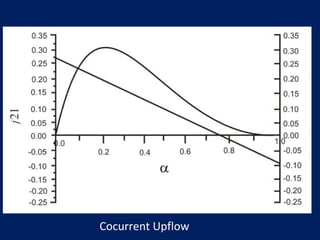
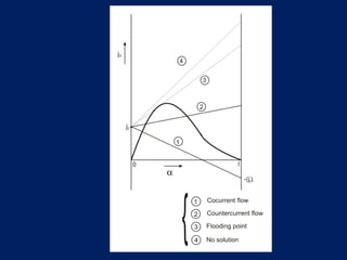
The drift flux model is applicable to two-phase flows like gas-liquid flows and fluidized beds. It accounts for the relative velocity between phases using the concept of drift flux. The model equations can be solved graphically or numerically to obtain void fraction and drift velocity for different flow regimes like cocurrent, countercurrent flows. Correlations are provided to estimate drift velocity and void profile parameter based on flow conditions.