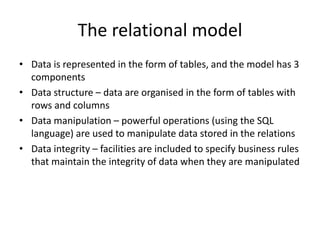
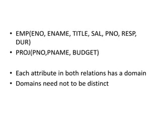
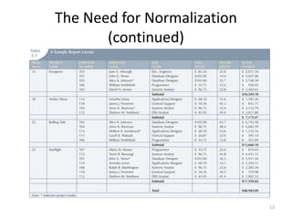
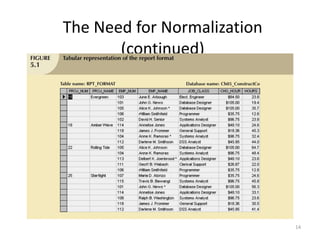
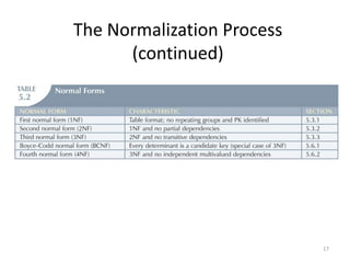
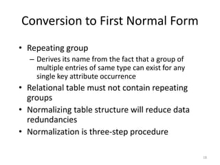
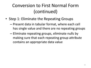
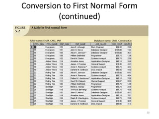
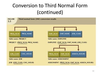
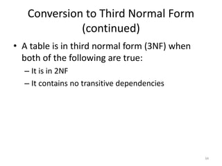
Background
Overview of Relational DBMS
Relational Data Model
• Two major strengths
• Three components
• Relation database based on Relational DM
The relational model
• Data is represented in the form of tables, and the model has 3
components
• Data structure – data are organised in the form of tables with
rows and columns
• Data manipulation – powerful operations (using the SQL
language) are used to manipulate data stored in the relations
• Data integrity – facilities are included to specify business rules
that maintain the integrity of data when they are manipulated
Relation
• EMP(ENO, ENAME, TITLE, SAL, PNO, RESP,
DUR)
• PROJ(PNO,PNAME, BUDGET)
• Each attribute in both relations has a domain
• Domains need not to be distinct
Database Table Keys
Definition:
A key of a relation is a subset of attributes with the
following attributes:
• Unique identification
• Non-redundancy
Relational Database Keys
Normalization of Database Tables
9
In this chapter, you will learn:
• What normalization is and what role it plays in the
database design process
• About the normal forms 1NF, 2NF, 3NF, BCNF,
and 4NF
• How normal forms can be transformed from lower
normal forms to higher normal forms
• How normalization and ER modeling are used
concurrently to produce a good database design
• How some situations require denormalization to
generate information efficiently
10
Database Tables and Normalization
• Normalization
– Process for evaluating and correcting table
structures to minimize data redundancies
• Reduces data anomalies
– Works through a series of stages called normal
forms:
• First normal form (1NF)
• Second normal form (2NF)
• Third normal form (3NF)
11
Database Tables and Normalization
(continued)
• Normalization (continued)
– 2NF is better than 1NF; 3NF is better than 2NF
– For most business database design purposes, 3NF
is as high as we need to go in normalization
process
– Highest level of normalization is not always most
desirable
12
The Need for Normalization
• Example: Company that manages building
projects
– Charges its clients by billing hours spent on each
contract
– Hourly billing rate is dependent on employee’s
position
– Periodically, report is generated that contains
information displayed in Table 5.1
13
The Need for Normalization
(continued)
14
The Need for Normalization
(continued)
15
The Need for Normalization
(continued)
• Structure of data set in Figure 5.1 does not
handle data very well
• The table structure appears to work; report
generated with ease
• Unfortunately, report may yield different
results depending on what data anomaly has
occurred
16
The Normalization Process
• Each table represents a single subject
• No data item will be unnecessarily stored in
more than one table
• All attributes in a table are dependent on the
primary key
17
The Normalization Process
(continued)
18
Conversion to First Normal Form
• Repeating group
– Derives its name from the fact that a group of
multiple entries of same type can exist for any
single key attribute occurrence
• Relational table must not contain repeating
groups
• Normalizing table structure will reduce data
redundancies
• Normalization is three-step procedure
19
Conversion to First Normal Form
(continued)
• Step 1: Eliminate the Repeating Groups
– Present data in tabular format, where each cell
has single value and there are no repeating groups
– Eliminate repeating groups, eliminate nulls by
making sure that each repeating group attribute
contains an appropriate data value
20
Conversion to First Normal Form
(continued)
21
Conversion to First Normal Form
(continued)
• Step 2: Identify the Primary Key
– Primary key must uniquely identify attribute value
– New key must be composed
22
Conversion to First Normal Form
(continued)
• Step 3: Identify All Dependencies
– Dependencies can be depicted with help of a
diagram
– Dependency diagram:
• Depicts all dependencies found within given table
structure
• Helpful in getting bird’s-eye view of all relationships
among table’s attributes
• Makes it less likely that will overlook an important
dependency
23
Conversion to First Normal Form
(continued)
24
Conversion to First Normal Form
(continued)
• First normal form describes tabular format in which:
– All key attributes are defined
– There are no repeating groups in the table
– All attributes are dependent on primary key
• All relational tables satisfy 1NF requirements
• Some tables contain partial dependencies
– Dependencies based on only part of the primary key
– Sometimes used for performance reasons, but should be
used with caution
– Still subject to data redundancies
25
Conversion to Second Normal Form
• Relational database design can be improved
by converting the database into second
normal form (2NF)
• Two steps
26
Conversion to Second Normal Form
(continued)
• Step 1: Write Each Key Component
on a Separate Line
– Write each key component on separate line, then
write original (composite) key on last line
– Each component will become key in new table
27
Conversion to Second Normal Form
(continued)
• Step 2: Assign Corresponding Dependent
Attributes
– Determine those attributes that are dependent on
other attributes
– At this point, most anomalies have been
eliminated
28
Conversion to Second Normal Form
(continued)
29
Conversion to Second Normal Form
(continued)
• Table is in second normal form (2NF) when:
– It is in 1NF and
– It includes no partial dependencies:
• No attribute is dependent on only portion of primary
key
30
Conversion to Third Normal Form
• Data anomalies created are easily eliminated
by completing three steps
• Step 1: Identify Each New Determinant
– For every transitive dependency, write its
determinant as PK for new table
• Determinant
– Any attribute whose value determines other values within a
row
31
Conversion to Third Normal Form
(continued)
• Step 2: Identify the Dependent Attributes
– Identify attributes dependent on each
determinant identified in Step 1 and identify
dependency
– Name table to reflect its contents and function
32
Conversion to Third Normal Form
(continued)
• Step 3: Remove the Dependent Attributes
from Transitive Dependencies
– Eliminate all dependent attributes in transitive
relationship(s) from each of the tables that have
such a transitive relationship
– Draw new dependency diagram to show all tables
defined in Steps 1–3
– Check new tables as well as tables modified in
Step 3 to make sure that each table has
determinant and that no table contains
inappropriate dependencies
33
Conversion to Third Normal Form
(continued)
34
Conversion to Third Normal Form
(continued)
• A table is in third normal form (3NF) when
both of the following are true:
– It is in 2NF
– It contains no transitive dependencies
Formal Relational Query Languages
• Two mathematical Query Languages form the
basis for “real” languages (e.g. SQL), and for
implementation:
– Relational Algebra: More operational, very
useful for representing execution plans.
– Relational Calculus: Lets users describe what
they want, rather than how to compute it.
(Non-operational, declarative.)
Example Instances
sid sname rating age
22 dustin 7 45.0
31 lubber 8 55.5
58 rusty 10 35.0
sid sname rating age
28 yuppy 9 35.0
31 lubber 8 55.5
44 guppy 5 35.0
58 rusty 10 35.0
sid bid day
22 101 10/10/96
58 103 11/12/96
R1
S1
S2
• “Sailors” and “Reserves”
relations for our
examples.
• We’ll use positional or
named field notation,
assume that names of
fields in query results are
`inherited’ from names of
fields in query input
relations.
Relational Algebra
• Basic operations:
– Selection ( ) Selects a subset of rows from relation.
– Projection ( ) Deletes unwanted columns from relation.
– Cross-product ( ) Allows us to combine two relations.
– Set-difference ( ) Tuples in reln. 1, but not in reln. 2.
– Union ( ) Tuples in reln. 1 and in reln. 2.
• Additional operations:
– Intersection, join, division, renaming: Not essential, but (very!)
useful.
• Since each operation returns a relation, operations can be composed!
(Algebra is “closed”.)





Projection
sname rating
yuppy 9
lubber 8
guppy 5
rusty 10
sname rating
S
,
( )2
age
35.0
55.5
age S( )2
• Deletes attributes that are not in
projection list.
• Schema of result contains exactly the
fields in the projection list, with the
same names that they had in the
(only) input relation.
• Projection operator has to eliminate
duplicates! (Why??)
– Note: real systems typically don’t
do duplicate elimination unless
the user explicitly asks for it.
(Why not?)
Selection
rating
S
8
2( )
sid sname rating age
28 yuppy 9 35.0
58 rusty 10 35.0
sname rating
yuppy 9
rusty 10
 sname rating rating
S
,
( ( ))
8
2
• Selects rows that satisfy
selection condition.
• No duplicates in result!
(Why?)
• Schema of result identical
to schema of (only) input
relation.
• Result relation can be the
input for another
relational algebra
operation! (Operator
composition.)
Union, Intersection, Set-Difference
• All of these operations take
two input relations, which
must be union-compatible:
– Same number of fields.
– `Corresponding’ fields have
the same type.
• What is the schema of result?
sid sname rating age
22 dustin 7 45.0
31 lubber 8 55.5
58 rusty 10 35.0
44 guppy 5 35.0
28 yuppy 9 35.0
sid sname rating age
31 lubber 8 55.5
58 rusty 10 35.0
S S1 2
S S1 2
sid sname rating age
22 dustin 7 45.0
S S1 2
Cross-Product
• Each row of S1 is paired with each row of R1.
• Result schema has one field per field of S1 and R1, with
field names `inherited’ if possible.
– Conflict: Both S1 and R1 have a field called sid.
 ( ( , ), )C sid sid S R1 1 5 2 1 1  
(sid) sname rating age (sid) bid day
22 dustin 7 45.0 22 101 10/10/96
22 dustin 7 45.0 58 103 11/12/96
31 lubber 8 55.5 22 101 10/10/96
31 lubber 8 55.5 58 103 11/12/96
58 rusty 10 35.0 22 101 10/10/96
58 rusty 10 35.0 58 103 11/12/96
 Renaming operator:
Joins
• Combine information from two or more tables
• Example: students enrolled in courses:
S1 S1.sid=E.studidE
Sid name gpa
50000 Dave 3.3
53666 Jones 3.4
53688 Smith 3.2
53650 Smith 3.8
53831 Madayan 1.8
53832 Guldu 2.0
cid grade studid
Carnatic101 C 53831
Reggae203 B 53832
Topology112 A 53650
History 105 B 53666
S1
E
Joins
sid name gpa cid grade studid
53666 Jones 3.4 History105 B 53666
53650 Smith 3.8 Topology112 A 53650
53831 Madayan 1.8 Carnatic101 C 53831
53832 Guldu 2.0 Reggae203 B 53832
Sid name gpa
50000 Dave 3.3
53666 Jones 3.4
53688 Smith 3.2
53650 Smith 3.8
53831 Madayan 1.8
53832 Guldu 2.0
cid grade studid
Carnatic101 C 53831
Reggae203 B 53832
Topology112 A 53650
History 105 B 53666
S1
E
Joins
• Condition Join:
• Result schema same as that of cross-product.
• Fewer tuples than cross-product, might be able to
compute more efficiently
• Sometimes called a theta-join.
R c S c R S   ( )
(sid) sname rating age (sid) bid day
22 dustin 7 45.0 58 103 11/12/96
31 lubber 8 55.5 58 103 11/12/96
S R
S sid R sid
1 1
1 1

. .
Joins
• Equi-Join: A special case of condition join where the condition c
contains only equalities.
• Result schema similar to cross-product, but only one copy of
fields for which equality is specified.
• Natural Join: Equijoin on all common fields.
sid sname rating age bid day
22 dustin 7 45.0 101 10/10/96
58 rusty 10 35.0 103 11/12/96
S R
sid
1 1
Division
• Not supported as a primitive operator, but useful for expressing
queries like:
Find sailors who have reserved all boats.
• Let A have 2 fields, x and y; B have only field y:
– A/B =
– i.e., A/B contains all x tuples (sailors) such that for every y tuple
(boat) in B, there is an xy tuple in A.
– Or: If the set of y values (boats) associated with an x value
(sailor) in A contains all y values in B, the x value is in A/B.
• In general, x and y can be any lists of fields; y is the list of fields in B,
and x y is the list of fields of A.
 x x y A y B| ,   

Examples of Division A/B
sno pno
s1 p1
s1 p2
s1 p3
s1 p4
s2 p1
s2 p2
s3 p2
s4 p2
s4 p4
pno
p2
pno
p2
p4
pno
p1
p2
p4
sno
s1
s2
s3
s4
sno
s1
s4
sno
s1
A
B1
B2
B3
A/B1 A/B2 A/B3
Expressing A/B using Basic Operators
• For A/B, compute all x values that are not
`disqualified’ by some y value in B.
– x value is disqualified if by attaching y value
from B, we obtain an xy tuple that is not in A.
Find names of sailors who’ve reserved boat
#103
• Solution 1:  sname bid
serves Sailors(( Re ) )
103

 Solution 2:  ( , Re )Temp serves
bid
1
103
 ( , )Temp Temp Sailors2 1
 sname Temp( )2
 Solution 3:  sname bid
serves Sailors( (Re ))
103

Find names of sailors who’ve reserved a red
boat
• Information about boat color only available in
Boats; so need an extra join:
 sname color red
Boats serves Sailors((
' '
) Re )

 
 A more efficient solution:
   sname sid bid color red
Boats s Sailors( ((
' '
) Re ) )

 
A query optimizer can find this, given the first solution!
Find sailors who’ve reserved a red or a green boat
• Can identify all red or green boats, then find
sailors who’ve reserved one of these boats:
 ( ,(
' ' ' '
))Tempboats
color red color green
Boats
  
 sname Tempboats serves Sailors( Re ) 
 Can also define Tempboats using union! (How?)
 What happens if is replaced by in this query? 
Find the names of sailors who’ve reserved all boats
• Uses division; schemas of the input relations to /
must be carefully chosen:
  ( , (
,
Re ) / ( ))Tempsids
sid bid
serves
bid
Boats
 sname Tempsids Sailors( )
 To find sailors who’ve reserved all ‘Interlake’ boats:
/ (
' '
) 
bid bname Interlake
Boats

.....
Other Relational Languages
• Relational calculus -tuple or domain (QBE)
• SQL -you already know!
Summary
• The relational model has rigorously defined query
languages that are simple and powerful.
• Relational algebra is more operational; useful as
internal representation for query evaluation plans.
• Several ways of expressing a given query; a query
optimizer should choose the most efficient version.

Distributed database

  • 1.
  • 2.
    Relational Data Model •Two major strengths • Three components • Relation database based on Relational DM
  • 3.
    The relational model •Data is represented in the form of tables, and the model has 3 components • Data structure – data are organised in the form of tables with rows and columns • Data manipulation – powerful operations (using the SQL language) are used to manipulate data stored in the relations • Data integrity – facilities are included to specify business rules that maintain the integrity of data when they are manipulated
  • 4.
  • 5.
    • EMP(ENO, ENAME,TITLE, SAL, PNO, RESP, DUR) • PROJ(PNO,PNAME, BUDGET) • Each attribute in both relations has a domain • Domains need not to be distinct
  • 6.
    Database Table Keys Definition: Akey of a relation is a subset of attributes with the following attributes: • Unique identification • Non-redundancy
  • 7.
  • 8.
  • 9.
    9 In this chapter,you will learn: • What normalization is and what role it plays in the database design process • About the normal forms 1NF, 2NF, 3NF, BCNF, and 4NF • How normal forms can be transformed from lower normal forms to higher normal forms • How normalization and ER modeling are used concurrently to produce a good database design • How some situations require denormalization to generate information efficiently
  • 10.
    10 Database Tables andNormalization • Normalization – Process for evaluating and correcting table structures to minimize data redundancies • Reduces data anomalies – Works through a series of stages called normal forms: • First normal form (1NF) • Second normal form (2NF) • Third normal form (3NF)
  • 11.
    11 Database Tables andNormalization (continued) • Normalization (continued) – 2NF is better than 1NF; 3NF is better than 2NF – For most business database design purposes, 3NF is as high as we need to go in normalization process – Highest level of normalization is not always most desirable
  • 12.
    12 The Need forNormalization • Example: Company that manages building projects – Charges its clients by billing hours spent on each contract – Hourly billing rate is dependent on employee’s position – Periodically, report is generated that contains information displayed in Table 5.1
  • 13.
    13 The Need forNormalization (continued)
  • 14.
    14 The Need forNormalization (continued)
  • 15.
    15 The Need forNormalization (continued) • Structure of data set in Figure 5.1 does not handle data very well • The table structure appears to work; report generated with ease • Unfortunately, report may yield different results depending on what data anomaly has occurred
  • 16.
    16 The Normalization Process •Each table represents a single subject • No data item will be unnecessarily stored in more than one table • All attributes in a table are dependent on the primary key
  • 17.
  • 18.
    18 Conversion to FirstNormal Form • Repeating group – Derives its name from the fact that a group of multiple entries of same type can exist for any single key attribute occurrence • Relational table must not contain repeating groups • Normalizing table structure will reduce data redundancies • Normalization is three-step procedure
  • 19.
    19 Conversion to FirstNormal Form (continued) • Step 1: Eliminate the Repeating Groups – Present data in tabular format, where each cell has single value and there are no repeating groups – Eliminate repeating groups, eliminate nulls by making sure that each repeating group attribute contains an appropriate data value
  • 20.
    20 Conversion to FirstNormal Form (continued)
  • 21.
    21 Conversion to FirstNormal Form (continued) • Step 2: Identify the Primary Key – Primary key must uniquely identify attribute value – New key must be composed
  • 22.
    22 Conversion to FirstNormal Form (continued) • Step 3: Identify All Dependencies – Dependencies can be depicted with help of a diagram – Dependency diagram: • Depicts all dependencies found within given table structure • Helpful in getting bird’s-eye view of all relationships among table’s attributes • Makes it less likely that will overlook an important dependency
  • 23.
    23 Conversion to FirstNormal Form (continued)
  • 24.
    24 Conversion to FirstNormal Form (continued) • First normal form describes tabular format in which: – All key attributes are defined – There are no repeating groups in the table – All attributes are dependent on primary key • All relational tables satisfy 1NF requirements • Some tables contain partial dependencies – Dependencies based on only part of the primary key – Sometimes used for performance reasons, but should be used with caution – Still subject to data redundancies
  • 25.
    25 Conversion to SecondNormal Form • Relational database design can be improved by converting the database into second normal form (2NF) • Two steps
  • 26.
    26 Conversion to SecondNormal Form (continued) • Step 1: Write Each Key Component on a Separate Line – Write each key component on separate line, then write original (composite) key on last line – Each component will become key in new table
  • 27.
    27 Conversion to SecondNormal Form (continued) • Step 2: Assign Corresponding Dependent Attributes – Determine those attributes that are dependent on other attributes – At this point, most anomalies have been eliminated
  • 28.
    28 Conversion to SecondNormal Form (continued)
  • 29.
    29 Conversion to SecondNormal Form (continued) • Table is in second normal form (2NF) when: – It is in 1NF and – It includes no partial dependencies: • No attribute is dependent on only portion of primary key
  • 30.
    30 Conversion to ThirdNormal Form • Data anomalies created are easily eliminated by completing three steps • Step 1: Identify Each New Determinant – For every transitive dependency, write its determinant as PK for new table • Determinant – Any attribute whose value determines other values within a row
  • 31.
    31 Conversion to ThirdNormal Form (continued) • Step 2: Identify the Dependent Attributes – Identify attributes dependent on each determinant identified in Step 1 and identify dependency – Name table to reflect its contents and function
  • 32.
    32 Conversion to ThirdNormal Form (continued) • Step 3: Remove the Dependent Attributes from Transitive Dependencies – Eliminate all dependent attributes in transitive relationship(s) from each of the tables that have such a transitive relationship – Draw new dependency diagram to show all tables defined in Steps 1–3 – Check new tables as well as tables modified in Step 3 to make sure that each table has determinant and that no table contains inappropriate dependencies
  • 33.
    33 Conversion to ThirdNormal Form (continued)
  • 34.
    34 Conversion to ThirdNormal Form (continued) • A table is in third normal form (3NF) when both of the following are true: – It is in 2NF – It contains no transitive dependencies
  • 35.
    Formal Relational QueryLanguages • Two mathematical Query Languages form the basis for “real” languages (e.g. SQL), and for implementation: – Relational Algebra: More operational, very useful for representing execution plans. – Relational Calculus: Lets users describe what they want, rather than how to compute it. (Non-operational, declarative.)
  • 36.
    Example Instances sid snamerating age 22 dustin 7 45.0 31 lubber 8 55.5 58 rusty 10 35.0 sid sname rating age 28 yuppy 9 35.0 31 lubber 8 55.5 44 guppy 5 35.0 58 rusty 10 35.0 sid bid day 22 101 10/10/96 58 103 11/12/96 R1 S1 S2 • “Sailors” and “Reserves” relations for our examples. • We’ll use positional or named field notation, assume that names of fields in query results are `inherited’ from names of fields in query input relations.
  • 37.
    Relational Algebra • Basicoperations: – Selection ( ) Selects a subset of rows from relation. – Projection ( ) Deletes unwanted columns from relation. – Cross-product ( ) Allows us to combine two relations. – Set-difference ( ) Tuples in reln. 1, but not in reln. 2. – Union ( ) Tuples in reln. 1 and in reln. 2. • Additional operations: – Intersection, join, division, renaming: Not essential, but (very!) useful. • Since each operation returns a relation, operations can be composed! (Algebra is “closed”.)     
  • 38.
    Projection sname rating yuppy 9 lubber8 guppy 5 rusty 10 sname rating S , ( )2 age 35.0 55.5 age S( )2 • Deletes attributes that are not in projection list. • Schema of result contains exactly the fields in the projection list, with the same names that they had in the (only) input relation. • Projection operator has to eliminate duplicates! (Why??) – Note: real systems typically don’t do duplicate elimination unless the user explicitly asks for it. (Why not?)
  • 39.
    Selection rating S 8 2( ) sid snamerating age 28 yuppy 9 35.0 58 rusty 10 35.0 sname rating yuppy 9 rusty 10  sname rating rating S , ( ( )) 8 2 • Selects rows that satisfy selection condition. • No duplicates in result! (Why?) • Schema of result identical to schema of (only) input relation. • Result relation can be the input for another relational algebra operation! (Operator composition.)
  • 40.
    Union, Intersection, Set-Difference •All of these operations take two input relations, which must be union-compatible: – Same number of fields. – `Corresponding’ fields have the same type. • What is the schema of result? sid sname rating age 22 dustin 7 45.0 31 lubber 8 55.5 58 rusty 10 35.0 44 guppy 5 35.0 28 yuppy 9 35.0 sid sname rating age 31 lubber 8 55.5 58 rusty 10 35.0 S S1 2 S S1 2 sid sname rating age 22 dustin 7 45.0 S S1 2
  • 41.
    Cross-Product • Each rowof S1 is paired with each row of R1. • Result schema has one field per field of S1 and R1, with field names `inherited’ if possible. – Conflict: Both S1 and R1 have a field called sid.  ( ( , ), )C sid sid S R1 1 5 2 1 1   (sid) sname rating age (sid) bid day 22 dustin 7 45.0 22 101 10/10/96 22 dustin 7 45.0 58 103 11/12/96 31 lubber 8 55.5 22 101 10/10/96 31 lubber 8 55.5 58 103 11/12/96 58 rusty 10 35.0 22 101 10/10/96 58 rusty 10 35.0 58 103 11/12/96  Renaming operator:
  • 42.
    Joins • Combine informationfrom two or more tables • Example: students enrolled in courses: S1 S1.sid=E.studidE Sid name gpa 50000 Dave 3.3 53666 Jones 3.4 53688 Smith 3.2 53650 Smith 3.8 53831 Madayan 1.8 53832 Guldu 2.0 cid grade studid Carnatic101 C 53831 Reggae203 B 53832 Topology112 A 53650 History 105 B 53666 S1 E
  • 43.
    Joins sid name gpacid grade studid 53666 Jones 3.4 History105 B 53666 53650 Smith 3.8 Topology112 A 53650 53831 Madayan 1.8 Carnatic101 C 53831 53832 Guldu 2.0 Reggae203 B 53832 Sid name gpa 50000 Dave 3.3 53666 Jones 3.4 53688 Smith 3.2 53650 Smith 3.8 53831 Madayan 1.8 53832 Guldu 2.0 cid grade studid Carnatic101 C 53831 Reggae203 B 53832 Topology112 A 53650 History 105 B 53666 S1 E
  • 44.
    Joins • Condition Join: •Result schema same as that of cross-product. • Fewer tuples than cross-product, might be able to compute more efficiently • Sometimes called a theta-join. R c S c R S   ( ) (sid) sname rating age (sid) bid day 22 dustin 7 45.0 58 103 11/12/96 31 lubber 8 55.5 58 103 11/12/96 S R S sid R sid 1 1 1 1  . .
  • 45.
    Joins • Equi-Join: Aspecial case of condition join where the condition c contains only equalities. • Result schema similar to cross-product, but only one copy of fields for which equality is specified. • Natural Join: Equijoin on all common fields. sid sname rating age bid day 22 dustin 7 45.0 101 10/10/96 58 rusty 10 35.0 103 11/12/96 S R sid 1 1
  • 46.
    Division • Not supportedas a primitive operator, but useful for expressing queries like: Find sailors who have reserved all boats. • Let A have 2 fields, x and y; B have only field y: – A/B = – i.e., A/B contains all x tuples (sailors) such that for every y tuple (boat) in B, there is an xy tuple in A. – Or: If the set of y values (boats) associated with an x value (sailor) in A contains all y values in B, the x value is in A/B. • In general, x and y can be any lists of fields; y is the list of fields in B, and x y is the list of fields of A.  x x y A y B| ,    
  • 47.
    Examples of DivisionA/B sno pno s1 p1 s1 p2 s1 p3 s1 p4 s2 p1 s2 p2 s3 p2 s4 p2 s4 p4 pno p2 pno p2 p4 pno p1 p2 p4 sno s1 s2 s3 s4 sno s1 s4 sno s1 A B1 B2 B3 A/B1 A/B2 A/B3
  • 48.
    Expressing A/B usingBasic Operators • For A/B, compute all x values that are not `disqualified’ by some y value in B. – x value is disqualified if by attaching y value from B, we obtain an xy tuple that is not in A.
  • 49.
    Find names ofsailors who’ve reserved boat #103 • Solution 1:  sname bid serves Sailors(( Re ) ) 103   Solution 2:  ( , Re )Temp serves bid 1 103  ( , )Temp Temp Sailors2 1  sname Temp( )2  Solution 3:  sname bid serves Sailors( (Re )) 103 
  • 50.
    Find names ofsailors who’ve reserved a red boat • Information about boat color only available in Boats; so need an extra join:  sname color red Boats serves Sailors(( ' ' ) Re )     A more efficient solution:    sname sid bid color red Boats s Sailors( (( ' ' ) Re ) )    A query optimizer can find this, given the first solution!
  • 51.
    Find sailors who’vereserved a red or a green boat • Can identify all red or green boats, then find sailors who’ve reserved one of these boats:  ( ,( ' ' ' ' ))Tempboats color red color green Boats     sname Tempboats serves Sailors( Re )   Can also define Tempboats using union! (How?)  What happens if is replaced by in this query? 
  • 52.
    Find the namesof sailors who’ve reserved all boats • Uses division; schemas of the input relations to / must be carefully chosen:   ( , ( , Re ) / ( ))Tempsids sid bid serves bid Boats  sname Tempsids Sailors( )  To find sailors who’ve reserved all ‘Interlake’ boats: / ( ' ' )  bid bname Interlake Boats  .....
  • 53.
    Other Relational Languages •Relational calculus -tuple or domain (QBE) • SQL -you already know!
  • 54.
    Summary • The relationalmodel has rigorously defined query languages that are simple and powerful. • Relational algebra is more operational; useful as internal representation for query evaluation plans. • Several ways of expressing a given query; a query optimizer should choose the most efficient version.