Contents
SQL
Power Query inExcel
Excel Functions for Data Preparation and Augmentation
SQL
Power Query in Excel
Excel Functions for Data Preparation and Augmentation
Data Retrieval, Preparation,Preprocessing,
ETL (Extract, Transform, Load), Wrangling,
Cleaning etc.
PROCESSES DESIGNED TO TRANSFORM RAW DATA INTO
MORE READILY USED FORMATS.
5.
Extract
> During dataextraction, raw data is copied or
exported from source locations to a staging area.
Data management teams can extract data from a
variety of data sources, which can be structured or
unstructured. Those sources include but are not
limited to:
◦ SQL or NoSQL servers
◦ CRM and ERP systems
◦ Flat files
◦ Email
◦ Web pages
Retrieve data from source
6.
Transform
> In thestaging area, the raw data undergoes data
processing. Here, the data is transformed and
consolidated for its intended analytical use case.
This phase can involve the following tasks:
◦ Filtering, cleansing, de-duplicating, validating, and
authenticating the data.
◦ Performing calculations, translations, or summarizations
based on the raw data. This can include changing row and
column headers for consistency, converting currencies or
other units of measurement, editing text strings, and more.
◦ Conducting audits to ensure data quality and compliance
◦ Removing, encrypting, or protecting data governed by
industry or governmental regulators
◦ Formatting the data into tables or joined tables to match the
schema of the target data warehouse.
Structure data for analysis
7.
Load
> In thislast step, the transformed data is moved
from the staging area into a target data warehouse.
Typically, this involves an initial loading of all data,
followed by periodic loading of incremental data
changes and, less often, full refreshes to erase and
replace data in the warehouse.
> For most organizations that use ETL, the process
is automated, well-defined, continuous and batch-
driven. Typically, ETL takes place during off-hours
when traffic on the source systems and the data
warehouse is at its lowest.
Load data into analytics software
8.
Data
Wrangling
> In additionto ETL, data
wrangling refers to enhancing
and adding to the
features/fields of a dataset.
> Addition of features/enriching
data can be done in both pre-
processing (ETL) (in Power
Query) and post-processing (in
Excel)
Why Learn SQL?
>Data in real-life most of the time does not come prepared. Often, a user
needs to access a database to retrieve data of their requirements. A
graduate of AIS needs a working knowledge of DBMS and SQL to be
able to independently retrieve data for analysis.
> It also enhances the understanding of AIS, as the backbone of an
AIS/ERP/CRM is a DBMS.
Database
> A databaseis an organized collection of data that is stored and
managed electronically, designed to facilitate easy access, retrieval, and
management of the data. Databases are structured to allow efficient
storage, modification, and querying of information, often using a
Database Management System (DBMS) to interact with the data.
DBMS Terminologies
Data CellValue
Record Row Tuple
Field Column Attribute
File Table Entity
Identifier Key Index
17.
Relational Model
> Therelational model is based on mathematical set theory and represents data as independent
relations. Each relation (table) is conceptually represented as a two-dimensional structure of
intersecting rows and columns. The relations are related to each other through the sharing of common
entity characteristics (values in columns).
> The relational model uses a collection of tables to represent both data and the relationships
among those data. Each table has multiple columns, and each column has a unique name. Tables
are also known as relations. The relational model is an example of a record-based model. Record-
based models are so named because the database is structured in fixed-format records of several
types. Each table contains records of a particular type. Each record type defines a fixed number of
fields, or attributes. The columns of the table correspond to the attributes of the record type. The
relational data model is the most widely used data model, and a vast majority of current database
systems are based on the relational model.
18.
Relationships
> One-to-many (1:Mor 1..*) relationship - Associations among two or more entities that
are used by data models. In a 1:M relationship, one entity instance is associated with
many instances of the related entity.
> Many-to-many (M:N or *..*) relationship - Association among two or more entities in
which one occurrence of an entity is associated with many occurrences of a related
entity and one occurrence of the related entity is associated with many occurrences of
the first entity.
> One-to-one (1:1 or 1..1) relationship - Associations among two or more entities that
are used by data models. In a 1:1 relationship, one entity instance is associated with
only one instance of the related entity.
Relational Database
> Arelational database is a structure that contains data about many categories
of information as well as the relationships between those categories.
> A relational database is a tabular form of database.
> Relational database management system (RDBMS) - A collection of
programs that manages a relational database. The RDBMS software translates
a user’s logical requests (queries) into commands that physically locate and
retrieve the requested data.
24.
Relational Database Design
GOALSFOR GOOD DESIGN
> Avoid data redundancy (repetition).
> Ensure data integrity and consistency.
> Enable easy data manipulation and
querying.
> Support scalability and future
modifications.
DATABASE NORMALIZATION FOR
GOOD DESIGN
> Normalization is the process of
organizing tables and their relationships
to minimize redundancy and
dependency.
◦ Reduce redundancy (e.g., no repeated
customer info in every order)
◦ Easier updates and deletions (no anomalies)
◦ Maintain data integrity
25.
Database
Normalization
Database normalization isthe systematic approach
to organizing data in a relational database to
minimize redundancy and dependency.
> First Normal Form (1NF)
> Second Normal Form (2NF)
> Third Normal Form (3NF)
> Boyce-Codd Normal Form (BCNF)
> Fourth Normal Form (4NF)
> Fifth Normal Form (5NF)
It is a refinement process for
producing the best possible data
structure.
The main goal is to divide large
tables into smaller, related tables
and link them through
relationships.
26.
Goal of (OLTP)Database
Normalization
> Each field of a table may only contain one item.
> All of the data in a column must mean the same thing.
> Each row of the table must be unique.
> A table must have no repeating columns.
> Each table must contain data about only one type of thing.
> There is no other non-key attribute that you would need to change in a table if
you changed another non-key attribute.
29.
1NF
> Rule:
◦ Eliminaterepeating groups (arrays or lists) by creating
separate rows.
◦ Table must not contain multi-valued attributes and must not
contain any repeating groups of attributes.
◦ Each field of a table may only contain one item.
◦ All of the data in a column must mean the same thing.
◦ Each row of the table must be unique.
◦ A table must have no repeating columns.
> Requirements:
◦ Each column contains atomic (indivisible) values.
◦ No repeating groups or arrays in a single column.
> Issue Solved:
◦ No comma separated values in a single column/field.
◦ Each cell to contain one single value.
30.
StudentID Name Subjects
1John Doe Math, Physics
2 Jane Smith Chemistry, Biology
Example:
StudentID Name Subject
1 John Doe Math
1 John Doe Physics
2 Jane Smith Chemistry
2 Jane Smith Biology
After 1NF:
31.
2NF
> Rule:
◦ Eliminatepartial dependencies (requires 1NF).
◦ Each non-key field must be about the same thing as the
primary key.
◦ Each table must contain data about only one type of thing –
functionally dependent things to be separated into a table.
> Requirements:
◦ Must be in 1NF.
◦ All non-key attributes must be fully dependent on the
primary key.
> Issue Solved:
◦ Eliminates redundancy caused by composite keys.
◦ Splits data into multiple tables based on full dependency.
◦ Provides scope for relationships among tables.
32.
> A partialdependency occurs when a non-key attribute is dependent on part
of a composite primary key rather than the whole key. E.g. Customer Name
and Customer Address is dependent on OrderID only and not on Product, even
though OrderID and Product together creates the composite primary key to
uniquely identify the record.
> Functional dependency is when a non-key attribute is dependent on a
primary key. E.g.: EmployeeID → EmployeeName (EmployeeName is
functionally dependent on EmployeeID).
33.
Example:
After 2NF:
OrderID ProductCustomerName CustomerAddress
101 Laptop Alice 123 Maple St
101 Tablet Alice 123 Maple St
102 Smartphone Bob 456 Oak Rd
OrderID Product CustomerID
101 Laptop 1
101 Tablet 1
102 Smartphone 2
CustomerID CustomerName CustomerAddress
1 Alice 123 Maple St
2 Bob 456 Oak Rd
34.
3NF
> Rule:
◦ Eliminatetransitive dependencies (requires 2NF).
◦ There is no other non-key attribute that you would need to
change in a table if you changed another non-key attribute.
> Requirements:
◦ Must be in 2NF.Non-key attributes must not depend on other
non-key attributes.
> Issue Solved:
◦ Prevents indirect dependency through another attribute.
35.
> A transitivedependency occurs when a non-key attribute depends on
another non-key attribute rather than directly on the primary key. E.g.: Course
→ Teacher ID → Teacher Name (Teacher Name is functionally dependent on
Teacher ID, which in turn is dependent on Course – this results in transitive
dependency where if course field was updated both Teacher ID and Teacher
Name would require updating. If Teacher ID was updated Teacher Name would
require updating which is not ideal).
36.
Example:
After 2NF:
StudentID StudentNameDepartment HOD
1 John CS Dr. Smith
2 Alice Math Dr. Brown
Department HOD
CS Dr. Smith
Math Dr. Brown
StudentID StudentName Department
1 John CS
2 Alice Math
Transitive
Dependency
Teacher Name isIndirectly Dependent on
Teacher ID, which in turn is Dependent on
Course Title. If Teacher was Changed Both
Name and ID would need to be updated.
Core Concepts: RDBMS
TermDescription
Table (Relation) Collection of related data organized in rows and columns
Row (Tuple) A single record in a table
Column (Attribute) A property or field of the table
Primary Key (PK) Uniquely identifies each row in a table
Foreign Key (FK) A key from one table that refers to the PK in another table
Entity A thing or object (e.g., Customer, Product)
Relationship Association between entities (1:1, 1:∞, ∞:∞)
47.
Database
vs Data
Warehouse
Feature DatabaseData Warehouse
Purpose
Day-to-day operations
(OLTP - Online Transaction
Processing)
Analytical processing and
reporting (OLAP - Online
Analytical Processing)
Data Type
Current, real-time,
transactional data
Historical, consolidated,
analytical data
Design Focus
Speed and accuracy for
CRUD operations (Create,
Read, Update, Delete)
Optimized for fast queries,
aggregation, and
summaries
Schema Design Highly normalized (3NF)
Denormalized/star/snowflak
e schema
Examples
MySQL, PostgreSQL, MS
Access, Oracle DB
Amazon Redshift, Google
BigQuery, Snowflake, MS
SQL DW
Data Sources
Usually one
application/system
Combines data from
multiple sources (CRM,
ERP, logs etc.)
Update Frequency Constant, frequent
Periodic (e.g., nightly,
weekly)
Users
Operations staff,
application users
Analysts, decision-makers,
data scientists
Structured Query Language
Languageused to construct and query data from relational databases
> DDL – Data Definition Language
◦ To construct and modify the database structure
> DML – Data Manipulation Language
◦ To read and modify data
> DQL – Data Query Language
◦ To read and query data (considered as part of DML)
> DCL – Data Control Language
> TCL – Transaction Control Language
50.
Which DBMS tolearn?
> MySQL
> PostgreSQL
> Oracle RDBMS
> Microsoft SQL Server
> Microsoft Access
> IBM Db2
51.
Basic SQL Keywords
(Commands)
>Syntax
◦ DDL, DML, DQL, DCL, TCL
> Constraints
> Operators
> Datatypes
> Functions
> Join
Keywords are written in BLOCK LETTERS. An SQL command ends with
a semi-colon;
52.
DDL - Keywords
>CREATE: Create a new database object.
◦ Example: CREATE TABLE Employees (...)
> ALTER: Modify an existing database object.
◦ Example: ALTER TABLE Employees ADD COLUMN Email VARCHAR(100)
> DROP: Delete a database object.
◦ Example: DROP TABLE Employees
53.
DML - Keywords
>SELECT: Query data from a table (DQL).
◦ Example: SELECT * FROM Employees
> INSERT: Insert new data into a table.
◦ Example: INSERT INTO Employees (FirstName, LastName) VALUES ('John', 'Doe')
> UPDATE: Update existing data within a table.
◦ Example: UPDATE Employees SET Salary = 65000 WHERE EmployeeID = 1
> DELETE: Delete data from a table.
◦ Example: DELETE FROM Employees WHERE EmployeeID = 1
54.
DCL - Keywords
>GRANT: Grant access rights to a user.
◦ Example: GRANT SELECT ON Employees TO user1
> REVOKE: Revoke access rights from a user.
◦ Example: REVOKE SELECT ON Employees FROM user1
55.
TCL - Keywords
>COMMIT: Save the changes made in a transaction.
◦ Example: COMMIT
> ROLLBACK: Revert the changes made in a transaction.
◦ Example: ROLLBACK
> SAVEPOINT: Set a savepoint within a transaction.
◦ Example: SAVEPOINT sp1
> RELEASE SAVEPOINT: Release a savepoint.
◦ Example: RELEASE SAVEPOINT sp1
56.
Logical Operators –Keywords
> WHERE: Filter records.
◦ Example: WHERE Salary > 50000
> AND: Combine multiple conditions.
◦ Example: WHERE FirstName = 'John' AND LastName = 'Doe'
> OR: Combine multiple conditions.
◦ Example: WHERE Salary > 50000 OR HireDate > '2020-01-01'
> NOT: Negate a condition.
◦ Example: WHERE NOT (Salary < 50000)
JOIN – Keywords
>JOIN: Combine rows from two or more tables.
◦ Example: SELECT * FROM Employees JOIN Departments ON Employees.DepartmentID = Departments.DepartmentID
> INNER JOIN: Return rows that have matching values in both tables.
◦ Example: SELECT * FROM Employees INNER JOIN Departments ON Employees.DepartmentID = Departments.DepartmentID
> LEFT JOIN: Return all rows from the left table, and matched rows from the right table.
◦ Example: SELECT * FROM Employees LEFT JOIN Departments ON Employees.DepartmentID = Departments.DepartmentID
> RIGHT JOIN: Return all rows from the right table, and matched rows from the left table.
◦ Example: SELECT * FROM Employees RIGHT JOIN Departments ON Employees.DepartmentID = Departments.DepartmentID
> FULL JOIN: Return all rows when there is a match in either table.
◦ Example: SELECT * FROM Employees FULL JOIN Departments ON Employees.DepartmentID = Departments.DepartmentID
59.
AGGREGATE – Functions
>COUNT: Return the number of rows.
◦ Example: SELECT COUNT(*) FROM Employees
> SUM: Return the sum of a numeric column.
◦ Example: SELECT SUM(Salary) FROM Employees
> AVG: Return the average value of a numeric column.
◦ Example: SELECT AVG(Salary) FROM Employees
> MIN: Return the smallest value.
◦ Example: SELECT MIN(Salary) FROM Employees
> MAX: Return the largest value.
◦ Example: SELECT MAX(Salary) FROM Employees
60.
String – Functions
>CONCAT(): Concatenates two or more strings.
◦ Example: SELECT CONCAT(FirstName, ' ', LastName) AS FullName FROM Employees;
> LENGTH(): Returns the length of a string.
◦ Example: SELECT LENGTH(FirstName) FROM Employees;
> UPPER(): Converts a string to uppercase.
◦ Example: SELECT UPPER(FirstName) FROM Employees;
> LOWER(): Converts a string to lowercase.
◦ Example: SELECT LOWER(FirstName) FROM Employees;
61.
> SUBSTRING(): Extractsa substring from a string.
◦ Example: SELECT SUBSTRING(FirstName, 1, 3) FROM Employees;
> TRIM(): Removes leading and trailing spaces from a string.
◦ Example: SELECT TRIM(FirstName) FROM Employees;
> REPLACE(): Replaces all occurrences of a substring within a string with another
substring.
◦ Example: SELECT REPLACE(FirstName, 'o', 'a') FROM Employees;
> LPAD() and RPAD(): Pads a string with another string to a specified length from the left
or right.
◦ Example: SELECT LPAD(FirstName, 10, '*') FROM Employees;
◦ Example: SELECT RPAD(FirstName, 10, '*') FROM Employees;
62.
Date and Time– Functions
> CURRENT_DATE(): Returns the current date.
◦ Example: SELECT CURRENT_DATE();
> CURRENT_TIME(): Returns the current time.
◦ Example: SELECT CURRENT_TIME();
> CURRENT_TIMESTAMP(): Returns the current date and time.
◦ Example: SELECT CURRENT_TIMESTAMP();
> DATE_ADD(): Adds a time interval to a date.
◦ Example: SELECT DATE_ADD(HireDate, INTERVAL 1 YEAR) FROM Employees;
63.
> DATE_SUB(): Subtractsa time interval from a date.
◦ Example: SELECT DATE_SUB(HireDate, INTERVAL 1 MONTH) FROM Employees;
> DATEDIFF(): Returns the number of days between two dates.
◦ Example: SELECT DATEDIFF(CURRENT_DATE(), HireDate) FROM Employees;
> EXTRACT(): Extracts a part of a date.
◦ Example: SELECT EXTRACT(YEAR FROM HireDate) FROM Employees;
> DAY(), MONTH(), YEAR(): Extracts the day, month, or year from a date.
◦ Example: SELECT DAY(HireDate), MONTH(HireDate), YEAR(HireDate) FROM Employees;
64.
Mathematical – Functions
>ABS(): Returns the absolute value of a number.
◦ Example: SELECT ABS(-5);
> CEIL(): Returns the smallest integer greater than or equal to a number.
◦ Example: SELECT CEIL(4.2);
> FLOOR(): Returns the largest integer less than or equal to a number.
◦ Example: SELECT FLOOR(4.8);
65.
> ROUND(): Roundsa number to a specified number of decimal places.
◦ Example: SELECT ROUND(4.567, 2);
> POWER(): Returns the value of a number raised to the power of another
number.
◦ Example: SELECT POWER(2, 3);
> SQRT(): Returns the square root of a number.
◦ Example: SELECT SQRT(16);
66.
Conditional – Functions
>COALESCE(): Returns the first non-null value in a list.
◦ Example: SELECT COALESCE(MiddleName, 'N/A') FROM Employees;
> NULLIF(): Returns NULL if the two specified expressions are equal.
◦ Example: SELECT NULLIF(DepartmentID, 0) FROM Employees;
67.
> CASE: Evaluatesa list of conditions and returns one of multiple possible result
expressions.
> Example:
SELECT
FirstName,
Salary,
CASE
WHEN Salary < 50000 THEN 'Low'
WHEN Salary BETWEEN 50000 AND 100000 THEN 'Medium'
ELSE 'High'
END AS SalaryRange
FROM Employees;
68.
Data Types
Data CategoryData Types
Numeric Datatypes INT: Integer data.
BIGINT: Large integer data.
SMALLINT: Small integer data.
TINYINT: Tiny integer data.
DECIMAL(p, s): Fixed-point number with precision p and scale s.
NUMERIC(p, s): Similar to DECIMAL.
FLOAT: Floating-point number.
REAL: Single-precision floating-point number.
String Datatypes CHAR(n): Fixed-length character string.
VARCHAR(n): Variable-length character string.
TEXT: Variable-length character string (large text data).
Date and Time
Datatypes
DATE: Date values (year, month, day).
TIME: Time values (hour, minute, second).
DATETIME: Date and time values.
TIMESTAMP: Timestamp values (usually includes time zone).
YEAR: Year values.
Binary Datatypes BINARY(n): Fixed-length binary data.
VARBINARY(n): Variable-length binary data.
BLOB: Binary large objects (large binary data).
Boolean Datatype BOOLEAN: True/False values.
69.
Data Types –
MSAccess
Data Category Data Types
Numeric
Datatypes
NUMBER
BYTE
INTEGER
LONG
CURRENCY
SINGLE
DOUBLE
COUNTER: Counts 1,2,3 – Auto assigns number
AUTOINCREMENT
String Datatypes VARCHAR(n): Variable-length character string.
TEXT: Variable-length character string (large text data).
MEMO
Date and Time
Datatypes
DATE: Date values (year, month, day).
TIME: Time values (hour, minute, second).
DATETIME: Date and time values.
TIMESTAMP: Timestamp values (usually includes time zone).
Binary
Datatypes
YESNO
70.
Constraints
Constraint Purpose
PRIMARY KEYEnsures each row has a unique identifier.
Example: EmployeeID INT PRIMARY KEY
FOREIGN KEY Ensures referential integrity between tables.
Example: FOREIGN KEY (DepartmentID)
REFERENCES Departments(DepartmentID)
NOT NULL Ensures a column cannot have a NULL value.
Example: LastName VARCHAR(50) NOT NULL
UNIQUE Ensures all values in a column are unique.
Example: Email VARCHAR(100) UNIQUE
CHECK Ensures all values in a column satisfy a specific
condition.
Example: Salary DECIMAL(10, 2) CHECK (Salary > 0)
DEFAULT Sets a default value for a column if none is provided.
Example: InStock BOOLEAN DEFAULT TRUE
71.
SQL – Best
Practice
>Readability
◦ Use Consistent Case for Keywords - SQL keywords should be
UPPERCASE.
◦ Use Proper Indentation & Line Breaks - Always format queries for
readability.
◦ Use Consistent Naming Conventions - Use PascalCase or snake_case
for table and column names.
◦ Indent the subquery and use parentheses for clarity.
> End queries with a semicolon (;)
> Use Single Quotes (' ') for Text & Hash (# #) for Dates
> Use AS for Aliases
> Place commas at the end of each column
> In INSERT statements, list values in the same order as columns
> Syntax/Keywords cannot be used as names
> Use TableName.ColumnName to refer to columns in SELECT
queries
CREATE - Example
CREATETABLE Employees (
EmployeeID INT PRIMARY KEY,
FirstName VARCHAR(50) NOT NULL,
LastName VARCHAR(50) NOT NULL,
HireDate DATE,
Salary DECIMAL(10, 2)
);
Syntax
Constraints, Functions, Conditional, Join
Datatypes
Table and Column Names
75.
CREATE – MSAccess
CREATE TABLE Employees (
EmployeeID INT PRIMARY KEY,
FirstName VARCHAR(50) NOT NULL,
LastName VARCHAR(50) NOT NULL,
HireDate DATE,
Salary NUMBER
);
Syntax
Constraints, Functions, Conditional, Join
Datatypes
Table and Column Names
76.
CREATE – MSAccess
CREATE TABLE Employees (
EmployeeID INT PRIMARY KEY,
FirstName VARCHAR(50) NOT NULL,
LastName VARCHAR(50) NOT NULL,
HireDate DATE,
Salary CURRENCY
);
Syntax
Constraints, Functions, Conditional, Join
Datatypes
Table and Column Names
77.
CREATE with FOREIGNKEY –
Example
CREATE TABLE Orders (
OrderID INT PRIMARY KEY,
OrderNumber INT NOT NULL,
EmployeeID INT NOT NULL,
FOREIGN KEY (EmployeeID) REFERENCES Employees(EmployeeID)
);
Syntax
Constraints, Functions, Conditional, Join
Datatypes
Table and Column Names
78.
CREATE with FOREIGNKEY –
MS Access
CREATE TABLE Orders (
OrderID INT PRIMARY KEY,
OrderNumber INT NOT NULL,
EmployeeID INT NOT NULL,
FOREIGN KEY (EmployeeID) REFERENCES Employees(EmployeeID)
);
Syntax
Constraints, Functions, Conditional, Join
Datatypes
Table and Column Names
Relationships
> One-to-many: Inone-to-many relationships, the linked attribute has unique
values in the original table, and non-unique/repeating values in the table linked
table.
> One-to-one: In one-to-one relationships, the linked attribute has unique values
in both the original and linked table.
◦ The attribute (original and FOREIGN KEY) has UNIQUE or PRIMARY KEY constraint on
both tables.
> Many-to-many: In many-to-many relationships, the linked attribute does not
have a unique value in any of the tables.
81.
One-to-One Relationship –
Example
CREATETABLE Employees (
EmployeeID INT PRIMARY KEY,
PhoneNo TEXT UNIQUE NOT NULL
);
CREATE TABLE EmployeeDetails (
EmployeeID INT PRIMARY KEY,
EmployeeName TEXT NOT NULL,
Address TEXT NOT NULL,
FOREIGN KEY (EmployeeID) REFERENCES Employees(EmployeeID)
);
ALTER
> Purpose: Tomodify an existing table.
> Syntax:
ALTER TABLE table_name
ADD column_name datatype constraint;
ALTER TABLE table_name
DROP column_name;
86.
ALTER TABLE table_name
MODIFYcolumn_name datatype constraint;
ALTER TABLE table_name
MODIFY COLUMN column_name datatype constraint;
ALTER TABLE table_name
RENAME COLUMN old_name new_name;
-- MS Access
ALTER TABLE table_name
ALTER COLUMN column_name datatype constraint;
ALTER TABLE table_name
ADD column_name datatype constraint;
ALTER TABLE table_name
DROP column_name;
87.
ALTER - Example
ALTERTABLE Employees
ADD Email VARCHAR(100);
ALTER TABLE Employees
ALTER COLUMN Email TEXT NOT NULL;
Syntax
Constraints, Functions, Conditional, Join
Datatypes
Table and Column Names
88.
DROP - Example
--Names the UNIQUE constraint as UQ_Email, so it can be dropped if needed.
ALTER TABLE Employees
ADD COLUMN Email TEXT NOT NULL CONSTRAINT UQ_Email UNIQUE;
ALTER TABLE Employees
DROP CONSTRAINT UQ_Email UNIQUE;
ALTER TABLE Employees
DROP COLUMN Email;
Syntax
Constraints, Functions, Conditional, Join
Datatypes
Table and Column Names
INSERT INTO
> Purpose:To insert new data into a table.
> Syntax:
INSERT INTO table_name (column1, column2, ...)
VALUES (value1, value2, ...);
91.
INSERT INTO -Example
INSERT INTO Employees (EmployeeID, FirstName, LastName,
HireDate, Salary)
VALUES (1, 'John', 'Doe', '2023-01-15', 60000.00);
INSERT INTO Orders (OrderID, OrderNumber, EmployeeID)
VALUES (1, 101, 1);
Syntax
Constraints, Functions, Conditional, Join
Datatypes
Table and Column Names
92.
INSERT INTO -Example
INSERT INTO Employees (EmployeeID, FirstName, LastName,
HireDate, Salary)
VALUES (1, 'John', 'Doe', #2023-01-15#, 60000.00);
INSERT INTO Orders (OrderID, OrderNumber, EmployeeID)
VALUES (1, 101, 1);
Syntax
Constraints, Functions, Conditional, Join
Datatypes
Table and Column Names
93.
Date Formats inMS Access
> MS Access requires dates to be enclosed with #
> When inserting data, dates can be:
◦ YYYY-MM-DD
◦ MM-DD-YYYY
◦ Windows regional settings
> When querying data, dates must be:
◦ MM-DD-YYYY
◦ Windows regional settings
94.
UPDATE
> Purpose: Toupdate existing data in a table.
> Syntax:
UPDATE table_name
SET column1 = value1, column2 = value2, ...
WHERE condition;
95.
UPDATE - Example
UPDATEEmployees
SET Salary = 100000
WHERE EmployeeID = 2;
UPDATE Employees
SET Salary = 1200000
WHERE FirstName = 'John';
Syntax
Constraints, Functions, Conditional, Join
Datatypes
Table and Column Names
96.
DELETE
> Purpose: Todelete existing data (record) from a table.
> Syntax:
DELETE FROM table_name
WHERE condition;
97.
DELETE - Example
DELETEFROM Employees
WHERE EmployeeID = 2;
Syntax
Constraints, Functions, Conditional, Join
Datatypes
Table and Column Names
98.
SELECT
> Purpose: Toquery data from a table.
> Syntax:
SELECT column1, column2, ...
FROM table_name
WHERE condition;
SELECT - Example
SELECTFirstName
FROM Employees;
SELECT FirstName AS EmployeeName
FROM Employees;
Syntax
Constraints, Functions, Conditional, Join
Datatypes
Table and Column Names
101.
SELECT - Example
SELECTFirstName, LastName, Salary
FROM Employees
WHERE Salary > 50000;
SELECT *
FROM Employees
WHERE Salary > 50000;
Syntax
Constraints, Functions, Conditional, Join
Datatypes
Table and Column Names
102.
Joining Tables inQuery
Joins are used to combine data from multiple tables based on a common field (or fields).
There are several types of joins:
1.Inner Join (default)
2.Left Join (Left Outer Join)
3.Right Join (Right Outer Join)
4.Full Outer Join (Not supported in MS Access)x
Typically, we JOIN on top of the table we are most interested in. That is:
FROM MainTable JOIN SupportingTable ON CommonField.
103.
INNER JOIN
> Aninner join returns only the rows where there is a match in both tables.
This is the default type of join when you use the INNER JOIN clause.
> Syntax:
SELECT table1.field1, table2.field2
FROM table1
INNER JOIN table2 ON table1.common_field =
table2.common_field;
table1 = main table, table2 = supporting table, common_field = foreign key/relationship
104.
INNER JOIN
> Supposeyou have two tables: Employees and Orders. You want to find
the names of employees who have processed orders. You would join the
two tables on EmployeeID (a field that exists in both tables).
SELECT
Employees.EmployeeID,
CONCAT(Employees.FirstName, ' ', Employees.LastName) AS EmployeeName,
Orders.OrderID
FROM
Employees
INNER JOIN Orders ON Employees.EmployeeID = Orders.EmployeeID;
105.
INNER JOIN –MS Access
> Suppose you have two tables: Employees and Orders. You want to find
the names of employees who have processed orders. You would join the
two tables on EmployeeID (a field that exists in both tables).
SELECT
Employees.EmployeeID,
Employees.FirstName & ' ' & Employees.LastName AS EmployeeName,
Orders.OrderID
FROM
Employees
INNER JOIN Orders ON Employees.EmployeeID = Orders.EmployeeID;
106.
SELECT - Example
SELECTEmployees.EmployeeID, Employees.FirstName AS
EmployeeName, Orders.OrderID, Orders.OrderNumber
FROM (Employees
INNER JOIN Orders ON Employees.EmployeeID =
Orders.EmployeeID)
WHERE Employees.EmployeeID = 1;
Syntax
Constraints, Functions, Conditional, Join
Datatypes
Table and Column Names
107.
Which Table toSelect Data From
> In an INNER JOIN, the main table (left table) (or the one you are
primarily querying from) should go in the FROM clause, while the table
you are joining (right table) is specified in the JOIN clause.
◦ The FROM table is typically the one with the most relevant data you need.
◦ The JOIN table is the one that adds extra details based on a matching condition.
The ‘Big
6’ ofSQL
Query
Criteria WHERE Clause HAVING Clause
Purpose
Filters rows before
aggregation.
Filters rows after
aggregation.
Used With
Works with
individual rows.
Works with grouped
or aggregated data.
Applicable To
Columns in the
table (individual
records).
Aggregated results
(e.g., SUM(), COUNT
()).
Stage of Query
Execution
Filters data
before GROUP
BY.
Filters data
after GROUP BY.
Aggregate
Functions
Cannot be used
with aggregate
functions.
Can be used with
aggregate functions.
> Set operationsare used to combine or compare results from two or more
queries. They work by applying operations to the results of queries as sets of
rows, meaning they treat the results as unordered collections of data. SQL
provides several set operations: UNION, INTERSECT, EXCEPT, and MINUS
(depending on the SQL dialect).
◦ Combine or compare results from multiple SELECT statements.
◦ They are typically used when you want to perform operations on entire result sets.
◦ They focus on manipulating the result sets rather than working with the underlying tables.
◦ They treat the results as distinct collections of rows and remove duplicates (except when
UNION ALL is used).
126.
> UNION: Combinestwo result sets, removing duplicates (or using UNION ALL to keep duplicates).
SELECT column1, column2, ...
FROM table1
UNION
SELECT column1, column2, ...
FROM table2;
> INTERSECT: Returns the common rows from two result sets.
SELECT column1, column2, ...
FROM table1
INTERSECT
SELECT column1, column2, ...
FROM table2;
> MINUS / EXCEPT: Returns rows from the first result set that are not in the second.
SELECT column1, column2, ...
FROM table1
EXCEPT
SELECT column1, column2, ...
FROM table2;
131.
Feature Sets Joins
Whatthey operate on Result sets (collections of rows) Tables (structure and rows)
Purpose Combine or compare result sets
Combine data from multiple tables
based on relationships
Output Distinct sets of rows
Combined rows based on
matching columns
Duplicates
Removes duplicates (except UNION
ALL)
Duplicates can exist, depending
on the type of join
Examples of Operations
UNION, INTERSECT, EXCEPT,
MINUS
INNER JOIN, LEFT JOIN, RIGHT
JOIN, FULL JOIN
Column Matching
No explicit column matching (results
from different queries)
Explicit column matching via ON
or USING clause
Use Case
Combining result sets from different
queries
Combining rows from different
tables based on a shared key
132.
SQL GROUP
BY
Groups outputbased on unique
input values. Can be used with
aggregate functions (sum, count
etc.). SELECT genre, SUM(qty) AS total
FROM books
GROUP BY genre;
133.
SQL and
Excel
Feature SQLExcel
Data Size
Handles millions of rows
efficiently
Struggles with large datasets
Data Storage
Stores data in relational
tables
Stores data in cells
Data Integrity
Enforces constraints and
relationships
No built-in data integrity
Querying
Uses SELECT, JOIN,
WHERE, etc.
Uses VLOOKUP, filters, pivot
tables
Performance Faster for large datasets Slower for complex operations
Automation
Uses stored procedures,
triggers
Uses VBA/macros
Security
Controlled access with
privileges
Less secure for large-scale
use
Excel Concept SQL Equivalent
Filtering with AutoFilter WHERE clause in SQL
Sorting data (Sort tool) ORDER BY
SUM, AVERAGE, COUNT SUM(), AVG(), COUNT()
PivotTables GROUP BY
VLOOKUP / INDEX + MATCH JOIN to combine tables
Store Database
> Thisdatabase contains information on employees, customers, products,
orders, and order details.
> This schema allows a DBMS user to query data find:
◦ Which employees fulfilled which order
◦ Which customer ordered which products
◦ Which order contains which products
◦ Etc.
137.
Schema
Table Name AttributesPrimary Key Foreign Key(s) Relationship
Employees
EmployeeID, FirstName, LastName,
HireDate, Salary
EmployeeID None
One-to-Many with
Orders
Customers
CustomerID, FirstName, LastName,
Address, Phone
CustomerID None
One-to-Many with
Orders
Products ProductID, ProductName, Price ProductID None
One-to-Many with
OrderDetails
Orders
OrderID, CustomerID, EmployeeID,
OrderDate, OrderDescription
OrderID
Customers
(CustomerID),
Employees
(EmployeeID)
One-to-Many with
OrderDetails,
Employees, Customers
OrderDetails
OrderDetailID, OrderID, ProductID,
Quantity
OrderDetailID
Orders (OrderID),
Products (ProductID)
One-to-Many with
Orders and Products
Orders
CREATE TABLE Orders(
OrderID INT PRIMARY KEY,
CustomerID INT NOT NULL,
EmployeeID INT NOT NULL,
OrderDate DATE NOT NULL,
OrderDescription TEXT,
FOREIGN KEY (CustomerID) REFERENCES Customers(CustomerID),
FOREIGN KEY (EmployeeID) REFERENCES Employees(EmployeeID)
);
143.
OrderDetails
CREATE TABLE OrderDetails(
OrderDetailID AUTOINCREMENT PRIMARY KEY,
OrderID INT NOT NULL,
ProductID INT NOT NULL,
Quantity INT NOT NULL,
FOREIGN KEY (OrderID) REFERENCES Orders(OrderID),
FOREIGN KEY (ProductID) REFERENCES Products(ProductID)
);
Products
ordered by a
specific
customer
SELECT
Customers.FirstNameAS CustomerName,
Products.ProductName,
OrderDetails.Quantity
FROM
(((Customers
INNER JOIN Orders ON Customers.CustomerID = Orders.CustomerID)
INNER JOIN OrderDetails ON Orders.OrderID = OrderDetails.OrderID)
INNER JOIN Products ON OrderDetails.ProductID = Products.ProductID)
WHERE
Customers.CustomerID = 1;
155.
Products ordered bya specific
customer
SELECT
Customers.FirstName AS CustomerName, Products.ProductName, OrderDetails.Quantity
FROM (((Customers
INNER JOIN Orders ON Customers.CustomerID = Orders.CustomerID)
INNER JOIN OrderDetails ON Orders.OrderID = OrderDetails.OrderID)
INNER JOIN Products ON OrderDetails.ProductID = Products.ProductID)
WHERE Customers.CustomerID = 1;
157.
Products ordered bya specific
customer
SELECT Customers.CustomerID, Customers.FirstName AS CustomerName,
Products.ProductName, OrderDetails.Quantity
FROM (((Customers INNER JOIN Orders ON Customers.CustomerID =
Orders.CustomerID) INNER JOIN OrderDetails ON Orders.OrderID =
OrderDetails.OrderID) INNER JOIN Products ON OrderDetails.ProductID =
Products.ProductID)
WHERE Customers.CustomerID = 1;
159.
Order Details includingCustomer info.
by Employee
SELECT
Employees.EmployeeID,
Employees.FirstName & ' ' & Employees.LastName AS EmployeeName,
Orders.OrderID,
Customers.FirstName & ' ' & Customers.LastName AS CustomerName,
Products.ProductName,
OrderDetails.Quantity,
Products.Price
FROM (((Employees
INNER JOIN Orders ON Employees.EmployeeID=Orders.EmployeeID)
INNER JOIN Customers ON Customers.CustomerID=Orders.CustomerID)
INNER JOIN OrderDetails ON OrderDetails.OrderID=Orders.OrderID)
INNER JOIN Products ON Products.ProductID=OrderDetails.ProductID;
Learning Outcomes
> Extractdata from structured/semi-structured files and automate basic transformations such
as Pivot and Unpivot.
> Identify the characteristics of good and bad data using the principles of data normalization.
> Load transformed data into Excel for use as automated data feeds.
> Extract information from fields that combine two or more values.
> Avoid, interpret and fix errors and exceptions that you experience in Power Query.
> Transform datasets by grouping or combining data from different tables, or even multiple
files from the same folder.
163.
SQL to
Excel
Using PowerQuery (Get Data) –
data can be retrieved from different
sources including files, database,
and online sources.
Accessing certain sources require
authorization/credentials.
Accessing certain database may
require installing specific
software/drivers.
165.
Power Query
(Get and
Transform)
>Extracts, Transforms, and Loads (ETL) data into
Excel from a range of data source.
> Records the steps and automates the process
for future usage.
> Allows appending/merging/grouping different
data sources.
> Offers tools for fixing errors and other
automation tools for your data.
166.
Principles of
Using Power
Query
>Recognize pattern of data
◦ Ensure the pattern remains consistent over following imports
(when you change source/import a new dataset of the same
purpose/origin/structure)
> Recognize pattern and sequence of steps
◦ Power Query will take the steps as you prescribe and in the
sequence you prescribe – literally. If the steps and sequence of
steps are not holistic (does not consider future
datasets/potential flexibility/dynamic nature/variation in
datasets) – power query will act in unexpected manners.
> One task can be performed in multiple ways
◦ Ensure whatever way is used works for all reasonable cases of
future imports.
> Understand purpose of data and analysis
◦ Purpose of data and type of analysis will dictate how you
process your data
167.
Power Query
Tools
> Home
◦Refresh
◦ Advanced Editor (M Code
Interface)
◦ Remove Columns
◦ Keep Rows, Remove Rows
◦ Sort
◦ Merge Queries
◦ Append Queries
◦ Data Source Settings
◦ New Source
> Transform
◦ Group By
◦ Use First Row as Headers
◦ Transpose
◦ Data Type
◦ Replace Values
◦ Fill
◦ Pivot
◦ Unpivot
◦ Convert to List
◦ Split Columns
◦ Format
◦ Extract
◦ Parse
◦ Merge
◦ Numeric Operations
> Add Columns
◦ Custom
◦ Conditional
◦ Calculated
◦ Index
◦ Duplicate
Data
Normalization
> Transforming datainto a more robust form for
storage and analysis
> Data normalization is the process of organizing
and transforming data to ensure consistency,
accuracy, and efficiency. It involves scaling data
values to a common range or format, reducing
redundancy, and improving data integrity.
◦ Improves data quality by reducing error and redundancies
◦ Facilitates analysis and comparison by structuring data in a
friendly manner
◦ Enhances performance by making data processes faster
and more efficient
172.
Usage of Normalization
>Database Normalization
◦ If a table contains StudentID, StudentName, Course, and Instructor, splitting this into two tables
(Students and Courses) eliminates redundancy.
> Statistical and Mathematical Normalization (Feature Scaling)
◦ Min-Max Normalization (Min value = 0, Max Value = 1)
◦ Z-Score Normalization (Standardization) based on mean or standard deviation (e.g.: 2 standard
deviation value)
◦ Decimal Scaling (moving the decimal point left or right)
◦ Log
> Text Data Normalization
◦ lowercase, UPPERCASE, Capitalize Each Word, PascalCase, Snake_Case: avoid case sensitivity
◦ Removing punctuation
◦ Stemming/Lemmatization: reducing words to root form (e.g., "running" → "run")
◦ Removing stop words: eliminates common words ("the", "is", etc.)
173.
Goal of DatabaseNormalization
in Power Query
1. Every attribute/value should have it’s own, single column.
◦ Each field of a table may only contain one item. Unpivot multi-columned same attribute to its own
singular column.
◦ No field should contain multiple value (no multivalued cells). Multivalued cells must be split into
their own rows.
◦ All of the data in a column must mean the same thing. Pivot values based on group/row labels, so
values of same meaning have their own column.
◦ Joined attribute must be split into their own columns.
2. Each row of the table must be unique.
3. A table must have no repeating columns.
174.
Rule 1 -Every attribute/value should have it’s own, single column.
175.
Basic
Transformation
> Loading Data
>Filtering
> Deduplication (Removing Duplicates)
> Removing/Splitting columns
◦ Blanks, Multivalued
> Deleting unwanted data/rows
◦ Blanks, Errors etc.
> Unpivot values
> Pivot values
> Grouping
> Cleaning
> Changing data type
176.
Ideal Power
Query Steps
1.Source Data
2. Check flexibility of query (in formula bar) – Futureproof query
◦ Check if there’s any column limitation set in the formula bar for the CSV import.
◦ Disable change type, remove already existing change type steps.
3. Remove unwanted rows and columns in a dynamic manner
◦ Remove top rows but filter out bottom/middle unwanted rows with a dynamic formula.
◦ Filter out/remove unwanted columns by keeping required columns
4. Fix grouped values, Replace values, Trim, Clean etc.
◦ Replace blanks with nulls
◦ Fill down group labels
5. Unpivot (Normalize Dataset), Pivot/Group, Extract, Split, Calculate
etc.
◦ Ensure split is also dynamic and future proof. Check formula for column references.
6. Change data type (should be the last step before loading)
7. Load
8. Test query with expanded dataset
The sequence of steps truly
depends on the data structure
and purpose. Conceptualize the
final output and organize your
steps/actions accordingly.
Typically, after importing data
the first goal is to normalize the
dataset
177.
Loading Data
to Excel
FromPower Query data can be
loaded into Excel as a Table, Pivot
Table, Pivot Chart, or the query
can be kept as a connection only
(without loading the data into an
excel worksheet).
• Close and Load
• Close and Load To…
178.
Caution on DifferentFile Types
> CSV
◦ Ensure the sourcing query does not limit the number of columns being imported.
Remove the limitation on no. of columns by editing the formula.
> Excel
◦ Ensure blank columns are removed in a dynamic manner. Select columns to keep and
then remove other columns.
179.
> = Csv.Document(File.Contents("D:PowerQuery FundamentalsDataPQ Exercise
1a.csv"),[Delimiter=",", Columns=19, Encoding=1252,
QuoteStyle=QuoteStyle.None])
Remove this to make CSV import dynamic (import as many columns as exists in
subsequent imports/source changes.
= Csv.Document(File.Contents("D:Power Query FundamentalsDataPQ Exercise
1a.csv"),[Delimiter=",", Encoding=1252, QuoteStyle=QuoteStyle.None])
180.
Remove other columnsinstead of remove blank columns to keep excel import
dynamic (ensure all blank columns are removed even if no. of blank columns
change).
181.
What if youhave variable
no. of columns to keep
and variable no. of
columns to remove
PROPOSE A SOLUTION
182.
Using an alreadycreated Query
> Duplicate: Duplicates a created query without keeping any connection
to the original file.
> Reference: Creates a new query which is linked to the referred one. Any
changes in referred will flow through to the new query.
> Loading: Load to table, pivot table, or just create connection.
Group Row Labels
toColumns (Pivot
Columns)
> Fix grouped row headers and pivot them to
have a column each.
> This ensures data normalization: One column
should not have multiple types of attribute.
185.
Pivot and Unpivotvs Transpose
> Pivot, Unpivot, and transpose are all ways to rotate tables, but they do it in
different ways. Pivot and Unpivot turns the table sideways and combines data,
while transpose just flips the table sideways without changing the data.
> Unpivot and Pivot are essentially ways to convert and combine horizontally
structured data into a vertically structured data and vise-versa.
> Transpose simply rotates rows to columns and columns to rows.
186.
Dynamic Filtering
> Forevery step is Power Query a formula/code is generated.
> Review the formula/code and ensure it would function even after
updating the dataset (even after the dataset naturally grows) –
accounting for different scenario.
> Some formula will require adding/removing code to ensure dynamic
behavior (error free functioning with the updating of dataset).
187.
Create filters wherefilter conditions are always met, even when the data
changes. In here, having it filter by First Character Q means – it will always keep
any value with First Character Q (e.g. Q1 XYZ, Q2 2020 etc.)
• If one chose to filter out 2018, 2019 etc. instead, then when data of 2020 is
loaded in, it won’t be filtered out.
• If one chose to filter in Q1,Q2,Q3,Q4 of 2018 and 2019, then when data of
2020 is loaded in, Q1,Q2,Q3,Q4 of 2020 won’t be filtered in.
188.
Working with Dates
>Date Datatype usually convert data that looks like a date to a date.
◦ 1/1/2025 to 01/01/2025
◦ 2025 to 01/01/2025
◦ Q1 2025 to Error
> Parse date can be used to convert data that are dates to date data type
◦ 1/1/2025 to 01/01/2025
◦ 2025 to Error
◦ Q1 2025 to Error
> Date Transform options allows extracting year, month, day from dates
> For Dates from Different Region, select Date Locale option in the data type to specify region.
189.
M Language
> Languageof Powery Query for ETL
◦ Each line of the code returns a new answer/a new transformation
◦ Each line of code builds on the last, and references the last line/step
◦ Add comma after each line to define a new step
◦ Add “//” before any text in a line to add comments to a code
> Refer to the formula bar to view the M code for each step
> Refer to the advanced editor to view the M code for the entire query
> Power Query M function reference - PowerQuery M | Microsoft Learn
190.
M query startswith the word “let” – allowing
users to define all the parts of the query
M query ends with the word “in” – which
indicates which step is the output/result of
the query
Comments on the code
Name of a step: #“StepXYZ”
191.
Extract Data
and Split
Columns
>From fields that combine two or more values
> Extract: Replaces the existing column with extracted
values or adds a new column with extracted values
◦ Length
◦ First/Last Character/Range
◦ Delimiter
> Split Columns: Splits one column into multiple columns
◦ Delimiter
◦ Number of characters
◦ Position
◦ UPPERCASE/lowercase
◦ Digit/Non-digit
> Split Columns into Rows: Splits columns with
multivalued cells into their own rows.
Tip:
1. Standardize/Clean delimiters
before splitting columns.
2. Make split columns dynamic
(by removing explicit mention
of separated columns in the
formula bar).
192.
Cleaning and
Standardizing
Data
> Trim:Removes unwanted/extra spaces (leading
and trailing spaces).
> Clean: Removes non-printing characters
> Replace Values: Replace values within cell or the
entire content of cell
> Format: Format data to lowercase, UPPERCASE,
or Capitalize Each Word, Add Prefix, Add Suffix
It is good practice to clean your
data from unwanted spaces,
non-printing characters, and
standardize your data to avoid
unexpected variations
Dynamic Split Columns
>= Table.SplitColumn(#"Uppercased Text", "Column4",
Splitter.SplitTextByDelimiter("|", QuoteStyle.Csv),
{"Column4.1", "Column4.2", "Column4.3", "Column4.4"})
Remove this to ensure data is split into as many columns as delimiters,
so that even when delimiters increase or decrease – the formula works,
and the correct number of columns are created.
196.
Consolidate
Data
> Grouping andAggregation
◦ Group (and aggregate) by Rows (Transform > Group by)
◦ Aggregate Similar Columns (Add column)
> Merging Tables - Perform Table Joins (similar
functionality to lookups/database joins): Pulling
data from another query based on lookup values
> Combining Identical Files – Combine data from
multiple excel files
◦ Files must have the same structure (same number of
header rows, same column headers, same data types)
> Extract info from file names
Group and combine data from
different sources.
Merging Tables
(Joins)
> MergingTables from multiple queries based
on common attribute – using Merge Queries
> Similar to Lookups and JOINS
199.
Combine
Identical
Files
> Combine fileswith similar
structure to pull data from
all of them.
◦ Modify individual files as
part of subquery (primary
transformations takes
place here)
◦ Complete the overall
combined file
Two ways to combine identical files:
• Combine and Transform
• Append Queries
200.
Combine and Transform
>New Query > From File > Folder
> Combine and Transform
> Edit the “Transform Sample File” to ETL the individual identical files.
> View the original query which should contain the combined identical files.
> This way has an advantage where only one identical file needs transforming,
and the final query also contains a source column so one can identify which
rows are from with source. It also automatically picks up new files as they are
placed in the source folder.
201.
Append Query
> Newquery for all the files separately.
> Append Query (or Append Query as New) > Select the tables (queries)
you want to append > They will be combined
> This method requires individually transforming the identical files as new
queries. The appended file also does not have any indication of source
(unless one is explicitly created during individual transformation
process).
202.
Dealing with
Errors and
Exceptions
>Filter Errors
> Calculated Columns and Conditional Columns
> Replacing a character to fix errors
> Different Regions of Dates
◦ Changing Date Column Locale
> Errors with File Locations: Parameters
Red bar in the column in PQ
indicates errors in data.
203.
Parameters
Custom input valuesthat can be
referred in the query formula (M
language). The parameters can
be changed without altering the
queries.
Use Case: Changing query
location/source of data
204.
Lists
> Converts valuesof a column to a list of values
◦ Select Column
◦ Transform > Convert to List
◦ Remove duplicates to keep unique list of values (make sure to remove errors
from the original column first for it to work)
> Usage: The list can be referred to in the query for: filtering and custom
columns using M language.
205.
Lookup with CustomColumns
> =Table[ColumnToReturn]{List.PositionOf(Table[ColumnToMatch],[ColumnToLook
Up])}
> =Categories[Category]{List.PositionOf(Categories[Acronym],[Cat])}
> This finds the position of [Cat] in Categories[Acronym], then returns
Categories[Category] from the same position. Similar to a Lookup.
> = Table.AddColumn(#“LastStep", "Category", each
Categories[Category]{List.PositionOf(Categories[Acronym],[Cat])})
207.
Count Distinct Valuesfor Each
Group with M
= Table.Group(#"Changed Type", {"EmployeeID", "EmployeeName"}, {{"Total Sales",
each List.Sum([Total]), type nullable number},{"Number of Orders", each
List.Count(List.Distinct([OrderID])), type number}})
Keywords
Keyword Purpose
let Beginvariable declarations
in Return final result
each Shorthand for row context (to dictate each row)
_ Current row value
if ... then ... else Conditional logic
null Represents no value
true/false Booleans
as Type declaration (optional)
type Define data type
error Raise an error
try ... otherwise Error handling
meta Add metadata to a value
Table
Function Purpose
Table.AddColumn
Adds anew column to a table based on a specified
formula.
Table.RemoveColumns Removes specified columns from a table.
Table.SelectRows Filters rows from a table based on a specified condition.
Table.AddRow Adds a new row to the table and appends it (to the end)
Table.InsertRow Adds a new row to the table in a specific position
Table.TransformColumn Transform an existing column based on a condition.
Table.Sort Sorts the rows of a table based on specified columns.
Table.Join Joins two tables based on common columns.
Table.Group
Groups rows in a table based on specified column(s),
applying aggregate functions.
Table.Pivot
Pivots rows of a table into columns, based on a key
column.
Table.UnpivotColumns Unpivots columns of a table into attribute-value pairs.
Table.ExpandRecordColumn
Expands columns containing records into multiple
columns.
Table.Buffer
Buffers a table in memory to improve performance in
certain scenarios.
214.
Table Functions
> Table.SelectRows
◦Table.SelectRows(table as table, condition as function) as table
◦ Table.SelectRows(SalesData, each [Amount] > 1000)
> Table.AddColumn
◦ Table.AddColumn(table as table, columnName as text, transformation as function) as
table
◦ Table.AddColumn(SalesData, "Discounted Price", each [Amount] * (1 -
[Discount]))
◦ Table.AddColumn(SalesData, "SalesLevel", each if [Amount] > 1000 then
"High" else "Low")
215.
> Table.TransformColumn
◦ Table.TransformColumns(table,transformOperations, optional defaultTransformation)
◦ Table.TransformColumns(Source, {{"Salary", each _ * 1.1}})
> Table.RemoveColumn
◦ Table.RemoveColumns(table as table, columns as list) as table
◦ Table.RemoveColumns(Source, {"RemoveThis"})
216.
> Table.AddRow
let
Source =Table.FromRecords({
[Name = "Alice", Age = 30],
[Name = "Bob", Age = 25]
}),
NewRow = [Name = "Charlie", Age = 35],
UpdatedTable = Table.AddRow(Source, NewRow)
in
UpdatedTable
217.
> Table.InsertRows
let
Source =Table.FromRecords({
[Name = "Alice", Age = 30],
[Name = "Bob", Age = 25]
}),
NewRow = [Name = "Charlie", Age = 35],
UpdatedTable = Table.InsertRows(Source, 2, {NewRow})
in
UpdatedTable
218.
Text
Function Purpose
Text.Contains Checksif a specified substring exists in a text value.
Text.End Returns the last N characters from a text string.
Text.Length Returns the number of characters in a text value.
Text.Lower Converts a text value to lowercase.
Text.Proper
Capitalizes the first letter of each word in the text
string.
Text.Replace
Replaces a specified substring within the text with a
new substring.
Text.ReplaceRange
Replaces a specified range (or portion) of a text
string with a new value.
Text.Reverse Reverses the order of characters in a text value.
Text.Start Returns the first N characters from a text string.
Text.Upper Converts a text value to uppercase.
Text.Trim
Removes any leading and trailing whitespace from a
text value.
219.
Text Functions
> Text.Contains
◦Text.Contains(text as nullable text, substring as text, optional comparer as nullable
function) as nullable logical
◦ Text.Contains("Power BI is cool", "BI")
◦ Output: true
> Text.Replace
◦ Text.Replace(text as nullable text, old as text, new as text) as nullable text
◦ Text.Replace("color", "or", "our")
◦ Output: colour
220.
> Text.ReplaceRange
◦ Text.ReplaceRange(textas text, offset as number, length as number, newText as text) as text
◦ Text.ReplaceRange("abcdef", 2, 3, "XYZ")
◦ Output: abXYZf
> Text.Replace with Conditions
◦ Table.TransformColumns(YourTable, {{"Product", each if [SalesAmount] > 1000
then Text.Replace(_, "Expensive", "Premium") else _, type text}})
◦ Output: For each sales greater than 1000, it replaces the value in Product (value of each
row represented with _ (underscore)) if the value is “Expensive” to “Premium”.
Otherwise keeps original value.
List
Function Purpose
List.Distinct
Removes duplicatevalues from a list, leaving
only distinct values.
List.Contains Checks if a specified value exists in a list.
List.Count Returns the count of items in a list.
List.Sort Sorts the items in a list.
List.Transform
Applies a specified transformation to each
element in a list.
List.First Returns the first item from a list.
List.Last Returns the last item from a list.
List.Generate
Generates a list by applying a function over a
specified range of values.
List.Accumulate
Performs an accumulation (reduction) on a list
using a function.
List.Sum Returns the sum of values in a list.
List.PositionOf
Used to find the position (index) of a specific
value in a list. It returns the zero-based index of
the first occurrence of the value.
223.
List Functions
> List.Contains
◦List.Contains(list as list, value as any, optional equationCriteria as any) as logical
◦ List.Contains({1, 2, 3}, 2)
◦ Output: true
> List.Distinct
◦ List.Distinct(list as list, optional equationCriteria as any) as list
◦ List.Distinct({"A", "B", "A", "C"})
◦ Output: { "A", "B", "C" }
224.
> List.Count
◦ List.Count(listas list) as number
◦ List.Count({1, 2, 3, 4, 5})
◦ Output: 5
> List.Count with Condition
◦ List.Count(List.Select(list, each condition))
◦ List.Count(List.Select({10, 20, 30, 60, 70, 80}, each _ > 50))
◦ Output: 3
225.
Lookup with CustomColumns
> =Table[ColumnToReturn]{List.PositionOf(Table[ColumnToMatch],[ColumnToLook
Up])}
> =Categories[Category]{List.PositionOf(Categories[Acronym],[Cat])}
> This finds the position of [Cat] in Categories[Acronym], then returns
Categories[Category] from the same position. Similar to a Lookup.
> = Table.AddColumn(#“LastStep", "Category", each
Categories[Category]{List.PositionOf(Categories[Acronym],[Cat])})
227.
Count Distinct Valuesfor Each
Group with M
= Table.Group(#"Changed Type", {"EmployeeID", "EmployeeName"}, {{"Total Sales",
each List.Sum([Total]), type nullable number},{"Number of Orders", each
List.Count(List.Distinct([OrderID])), type number}})
Record
Function Purpose
Record.FieldValues Returnsa list of the values in a record.
Record.AddField Adds a new field to an existing record.
Record.RemoveField Removes a specified field from a record.
Record.TransformFields
Applies a transformation to specific
fields in a record.
Record.ToTable
Converts a record into a table where
each field is converted into a row.
Record.FieldNames Returns a list of field names in a record.
Record.SelectFields
Selects specific fields from a record,
returning a new record.
233.
Record Function
> Record.AddField
◦Record.AddField(record as record, fieldName as text, fieldValue as any) as record
◦ Record.AddField([Name = "Alice", Age = 30], "LoyaltyStatus", "Gold")
◦ Output: [Name = "Alice", Age = 30, LoyaltyStatus = "Gold"]
> Record.SelectFields
◦ Record.SelectFields(record as record, fieldNames as list) as record
◦ Record.SelectFields([Name = "Alice", Age = 30, Address = "123 Maple
St"], {"Name", "Age"})
◦ Output: [Name = "Alice", Age = 30]
234.
> Record.RemoveField
◦ Record.RemoveField(recordas record, fieldName as text) as record
◦ Record.RemoveField([Name = "Alice", Age = 30, Address = "123 Maple St"],
"Address")
◦ Output: [Name = "Alice", Age = 30]
Data
Augmentation
> Based onthe purpose of analysis, an analyst might
be required to add additional features to a dataset.
E.g.: Adding a postcode column based on location,
Adding a prefix based on marital status etc.
> Data augmentation can be done in both Power
Query and Excel.
◦ Augmentation can be queries more complicated.
◦ Might require creating custom/conditional columns and
writing code.
> It is much easier/intuitive to augment data in Excel.
◦ Allows using traditional excel formula.
◦ If you want to preserve these augmentations/excel formula,
you can lock the calculation cells or import the augmented
excel file as another query.
Data augmentation or data
enriching means enhancing the
features of the dataset by adding
new attributes/variables (derived
from/based on) existing
attributes/variables.
237.
Excel
Functions
Text Functions
Date Functions
LogicalFunctions
Lookup Functions
Custom Functions
These functions can be used for data
preparation (ETL) as well as
augmentation.
ETL should preferably be done in
Power Query, as PQ stores all the
steps as code, as well as the source
file path, which can be easily modified
to suit future needs and updated
datasets. Excel formula does not allow
for similar flexibility.
Tips in usingText Functions
> Glance through the dataset
> Identify patterns and hidden structures
> Identify anomalies
> Construct functions to leverage patterns and anomalies
243.
Combine Data
> =CONCAT(text1,[text2]…)
> =TEXTJOIN(delimiter, ignore_empty, text1, [text2]…)
> & Operator (all cells must be selected individually to join)
Payment_No Bank_No
Invoice Month
PONumber,
Location First Letter,
Full Location
=MID(G2,4,LEN(G2)-10)
=MID(G2,4,FIND("-",G2,4)-4)
Do it with TEXTSPLIT as well.
CLEAN, TRIM,
UPPER
=SUBSTITUTE(F2,"S","")
=SUBSTITUTE(SUBSTITUTE(F2,"S",""),MID(F2,2,1),"")
=VALUE(SUBSTITUTE(SUBSTITUTE(F2,"S",""),MID(F2,2,1),""))
=VALUE(SUBSTITUTE(SUBSTITUTE(F2,"S",""),UNICHAR(160),""))
Date Functions inExcel
> TEXT
> NOW
> TODAY
> DATE
> DAY
> MONTH
> YEAR
> YEARFRAC
> DAYS
> DAYS360
> EOMONTH
> EDATE
> WORKDAY
> WORKDAY.INTL
> NETWORKDAYS
> NETWORKDAYS.INTL
> TIME
> TIMEVALUE
> WEEKDAY
> WEEKNUM
> ISOWEEKNUM
250.
Date Format inExcel
> Dates are numbers formatted to look like
dates.
◦ 1 is 1/1/1900
◦ Adding 1 increases date by 1 day
◦ 8th February 2023 is 44965 (Ctrl+;)
d 8 m 2 yy 23
dd 08 mm 02 yyyy 2023
ddd Wed mmm Feb
dddd Wednesday mmmm February
251.
> =TEXT(value, format_text)
◦Convert a value to a text (e.g., date value to date text)
> =DATE(year, month, date)
◦ Create a Date
> =DAY(serial)
◦ Returns the Day from a Date (or any text that looks like a date)
> =MONTH(serial)
◦ Returns the Month from a Date (or any text that looks like a date)
> =YEAR(serial)
◦ Returns the Year from a Date (or any text that looks like a date)
252.
> =EOMONTH(start_date, months)
◦Find the last day of a month a certain number of months before or after a given date.
> =EDATE(start_date, months)
◦ Move a certain number of months before or after a given date.
> =YEARFRAC(start_date, end_date, [basis])
◦ Returns the year fraction representing the number of days between start date & end date.
> =DAYS(end_date, start_date)
◦ Returns the number of days between two dates
> =DAYS360(end_date, start_date)
◦ Returns the number of days between two dates based on a 360 Day year (12, 30-day monts)
253.
> =WORKDAY(start_date, days,[holidays])
◦ Find the next workday before or after a given date. This excludes weekends and holidays. Saturday
& Sunday weekends. (days argument must be at least 1)
> =WORKDAY.INTL(start_date, days, [weekend], [holidays])
◦ Find the next workday before or after a given date. This excludes weekends and holidays. You can
specify the weekend dates as well. E.g., “0000110” – Friday, Saturday weekend.
> =NETWORKDAYS(start_date, end_date, [holidays])
◦ Find the number of workdays between 2 dates. This excludes weekends and holidays. Saturday &
Sunday weekends.
> =NETWORKDAYS.INTL(start_date, end_date, [weekend], [holidays])
◦ Find the number of workdays between 2 dates. This excludes weekends and holidays. You can
specify the weekend dates as well.
254.
TEXT DAY
DAYS, NETWORKDAYS,
NETWORKDAYS.INTL
TODAY
NOW
Duein 6 days
Due in 6
working days
+6, WORKDAYS, WORKDAYS.INTL
with Holidays list, EOMONTH
=WORKDAY.INTL(D5,6,"0100001",DATE(2020,4,10))
Due in 5
working days
into the next
month
=WORKDAY.INTL(EOMONTH(D5,0),5,"0100001",Holidays)
Due in one
month
=WORKDAY.INTL(EDATE(D5,1)-1,1,"0100001",Holidays)
Logical Functions inExcel
> IF
> IFS
> COUNTIFS
> SUMIFS
> AVERAGEIFS
> AND
> OR
> XOR
> NOT
> IFERROR
> IFNA
> SWITCH
258.
IF
> The IFfunction is a premade function in Excel, which returns values based on
a true or false condition.
> It is typed =IF and has 3 parts:
◦ =IF(logical_test, [value_if_true], [value_if_false])
◦ Logical_test (required argument) – This is the condition to be tested and evaluated as
either TRUE or FALSE.
◦ Value_if_true (optional argument) – The value that will be returned if the logical_test
evaluates to TRUE.
◦ Value_if_false (optional argument) – The value that will be returned if the logical_test
evaluates to FALSE
> For Numberswe can test:
◦ >, <, >=, <=, =, <>, “”
> For Text we can test:
◦ A1=“Text”
263.
Nested IF IFS
>The IFS function is a premade function in Excel, which returns values
based on one or more true or false conditions.
> It is typed =IFS and has two or more parts:
◦ =IFS(logical_test1, value_if_true1, [logical_test2, value_if_true2],
[logical_test3; ...)
◦ The conditions are referred to as logical_test1, logical_test2, ...
◦ Each condition relates to a return value.
264.
COUNTIFS
> The COUNTIFSfunction is a premade function in Excel, which counts
cells in a range based on one or more true or false condition.
> It is typed =COUNTIFS:
◦ =COUNTIFS(criteria_range1, criteria1, [criteria_range2, criteria2],
...)
◦ The conditions are referred to as critera1, criteria2, .. and so on
◦ The criteria_range1, criteria_range2, and so on, are the ranges where the
function check for the conditions.
COUNTIFS with Numbers
CriteriaFormula Example Description
Count if greater than =COUNTIF(range,">5") Count cells where value is
greater than 5.
Count if less than =COUNTIF(range,"<5") Count cells with values less than
5.
Count if equal to =COUNTIF(range,"=5") Count cells where value is equal
to 5.
Count if not equal to =COUNTIF(range,"<>5") Count cells where value is not
equal to 5.
Count if greater than or equal to =COUNTIF(range,">=5") Count cells where value is
greater than or equal to 5.
Count if less than or equal to =COUNTIF(range,"<=5") Count cells where value is less
than or equal to 5.
267.
COUNTIFS with Dates
CriteriaFormula Example Description
Count dates equal to the
specified date.
=COUNTIF(range,"6/1/2014") Counts the number of cells in
the range B2:B10 with the date
1-Jun-2014.
Count dates greater than
or equal to another date.
=COUNTIF(range,">=6/1/2014") Count the number of cells in
the range B2:B10 with a date
greater than or equal to
6/1/2014.
Count dates greater than
or equal to a date in
another cell, minus x days.
=COUNTIF(range,">="&B2-"7") Count the number of cells in
the range B2:B10 with a date
greater than or equal to the
date in B2 minus 7 days.
268.
COUNTIFS with Texts
>=COUNTIF(range,"??own")
> =COUNTIF(range,"Mr??????")
> =COUNTIF(range, "*Brown*")
> =COUNTIF(range,"Mr*")
> =COUNTIF(range,"*ed")
Tip. To find the number of cells containing an actual question mark or asterisk, type a tilde (~)
before the ? or * character in the formula. For example, =COUNTIF(range,"*~?*") will count all
cells containing the question mark in the range D2:D9.
269.
Misc. COUNTIFS
> =COUNTIF(range,"*")– Non-blank Text Cells
> =COUNTIF(range,"<>") – All Non-blank Cells
> =COUNTIF(range,"<>"&"") – All Non-blank Cells
> COUNTIF(range,"<>"&"*") – Not Containing Text
> COUNTIF(range,"") – All blank cells
> =COUNTBLANK(range)
> =ROWS(range)*COLUMNS(range)-COUNTBLANK(range)
> =COUNTIF(range,"=") – count excluding cells with empty strings
270.
SUMIFS
> The SUMIFSfunction is a premade function in Excel, which calculates
the sum of a range based on one or more true or false condition.
> It is typed =SUMIFS:
◦ =SUMIFS(sum_range, criteria_range1, criteria1, [criteria_range2,
criteria2] ...)
◦ The conditions are referred to as criteria1, criteria2, and so on.
◦ The [sum_range] is the range where the function calculates the sum.
271.
AVERAGEIFS
> The AVERAGEIFSfunction is a premade function in Excel, which calculates
the average of a range based on one or more true or false condition.
> It is typed =AVERAGEIFS:
◦ =AVERAGEIFS(average_range, criteria_range1, criteria1, ...)
◦ The conditions are referred to as critera1, criteria2, .. and so on
◦ The criteria_range1, criteria_range2, and so on, are the ranges where the
function check for the conditions.
◦ The average_range is the range where the function calculates the average.
272.
AND
> The ANDfunction is a premade function in Excel, which returns TRUE or
FALSE based on two or more conditions.
> It is typed =AND and takes two or more conditions.
◦ =AND([logical1], [logical2], ...)
◦ The conditions are referred to as [logical1], [logical2], and so on.
273.
Formula Description
=AND(A2="Bananas", B2>C2)
ReturnsTRUE if A2 contains "Bananas" and B2
is greater than C2, FALSE otherwise.
=AND(B2>20, B2=C2)
Returns TRUE if B2 is greater than 20 and B2 is
equal to C2, FALSE otherwise.
=AND(A2="Bananas", B2>=30, B2>C2)
Returns TRUE if A2 contains "Bananas", B2 is
greater than or equal to 30 and B2 is greater
than C2, FALSE otherwise.
274.
OR
> The ORfunction is a premade function in Excel, which returns TRUE or
FALSE based on two or more conditions.
> It is typed =OR.
◦ =OR([logical1], [logical2], ...)
◦ The conditions are referred to as [logical1], [logical2], and so on.
275.
Formula Description
=OR(A2="Bananas", A2="Oranges")
ReturnsTRUE if A2 contains "Bananas" or
"Oranges", FALSE otherwise.
=OR(B2>=40, C2>=20)
Returns TRUE if B2 is greater than or equal to
40 or C2 is greater than or equal to 20, FALSE
otherwise.
=OR(B2=" ", C2="")
Returns TRUE if either B2 or C2 is blank or
both, FALSE otherwise.
276.
XOR
> The XORin Excel, which returns TRUE only if one of the conditions are
met.
> It is typed =XOR.
◦ =XOR([logical1], [logical2], ...)
◦ The conditions are referred to as [logical1], [logical2], and so on.
◦ TRUE if either argument evaluates to TRUE.
◦ FALSE if both arguments are TRUE or neither is TRUE.
277.
Formula Result Description
=XOR(1>0,2<1) TRUE
Returns TRUE because the 1st
argument is TRUE and the
2nd argument is FALSE.
=XOR(1<0, 2<1) FALSE
Returns FALSE because both
arguments are FALSE.
=XOR(1>0, 2>1) FALSE
Returns FALSE because both
arguments are TRUE.
278.
NOT
> You usethe NOT function in Excel to reverse a value of its argument. In
other words, if logical evaluates to FALSE, the NOT function returns
TRUE and vice versa.
> It is typed =NOT.
◦ =NOT(logical)
279.
> If thelogical
statement is TRUE, it
returns FALSE
280.
Function Description FormulaExample Formula Description
AND
Returns TRUE if all of the
arguments evaluate to TRUE.
=AND(A2>=10, B2<5)
The formula returns TRUE if a value in cell A2
is greater than or equal to 10, and a value in B2
is less than 5, FALSE otherwise.
OR
Returns TRUE if any argument
evaluates to TRUE.
=OR(A2>=10, B2<5)
The formula returns TRUE if A2 is greater than
or equal to 10 or B2 is less than 5, or both
conditions are met. If neither of the conditions it
met, the formula returns FALSE.
XOR
Returns a logical Exclusive Or
of all arguments.
=XOR(A2>=10, B2<5)
The formula returns TRUE if either A2 is
greater than or equal to 10 or B2 is less than 5.
If neither of the conditions is met or both
conditions are met, the formula returns FALSE.
NOT
Returns the reversed logical
value of its argument. I.e. If the
argument is FALSE, then TRUE
is returned and vice versa.
=NOT(A2>=10)
The formula returns FALSE if a value in cell A1
is greater than or equal to 10; TRUE otherwise.
281.
IFERROR
> Instead ofthe resulting error, we can use IFERROR to return a
customized message such as “Invalid input.”
> It is typed =IFERROR.
◦ =IFERROR(value,value_if_error)
◦ Value (required argument) – This is the expression or value that needs to be tested. It
is generally provided as a cell address.
◦ Value_if_error (required argument) – The value that will be returned if the formula
evaluates to an error.
282.
> IFERROR +VLOOKUP
Function
> A very common use of
IFERROR function is with
the VLOOKUP function,
where it is used to point out
values that can’t be found.
283.
IFNA
> The purposeof the IFNA function is to use an alternate value instead of
the #N/A error.
> It is typed =IFNA.
◦ =IFNA(value,value_if_na)
◦ Value (required argument) – This is the formula or expression to be checked for an
#N/A error.
◦ Value_if_na (required argument) – This provides the specified value if the result of
the formula or expression is N/A error.
284.
> IFNA +VLOOKUP Function
> IFNA function tested the
results of VLOOKUP function.
VLOOKUP returned the #N/A
error value as it couldn’t find
Banana in the given lookup
range. However, IFNA
returned the value 0 in the cell
instead of the standard #N/A
error value.
285.
Using IFS insideother Functions
> What if you want to use logical functions for calculations other than
SUM, COUNT, AVERAGE?
> Nest IFS in that other function and write an array formula
(Ctrl+Shift+Enter).
> {=OTHERFUNCTION(IF(logical_test,rangetoreturn))}
> {=OTHERFUNCTION(IF(range=cell,rangetoreturn))}
In Excel 365, you don’t have to press Ctrl+Shift+Enter when completing formula to perform array
calculations, as it automatically recognizes array calculations.
286.
Nested IF IFAND
IFS OR IFNA
COUNTIFS
SUMIFS
AVERAGEIF
S
Lookup Functions inExcel
> CHOOSE
> HLOOKUP
> VLOOKUP
> INDEX
> MATCH
> XMATCH
> XLOOKUP
> FILTER
290.
=CHOOSE(index_num, value1, [value2],...)
• Index_num - Required. Specifies which value argument is selected. Index_num must
be a number between 1 and 254, or a formula or reference to a cell containing a
number between 1 and 254.
• If index_num is 1, CHOOSE returns value1; if it is 2, CHOOSE returns value2; and so on.
• If index_num is less than 1 or greater than the number of the last value in the list, CHOOSE
returns the #VALUE! error value.
• If index_num is a fraction, it is truncated to the lowest integer before being used.
• Value1, value2, ... - Value 1 is required, subsequent values are optional. 1 to
254 value arguments from which CHOOSE selects a value or an action to perform
based on index_num. The arguments can be numbers, cell references, defined names,
formulas, functions, or text.
291.
=VLOOKUP (lookup_value, table_array,col_index_num, [range_lookup])
Argument name Description
lookup_value
(required)
The value you want to look up. The value you want to look up must be in
the first column of the range of cells you specify in
the table_array argument.
For example, if table-array spans cells B2:D7, then your lookup_value
must be in column B.
Lookup_value can be a value or a reference to a cell.
table_array (required) The range of cells in which the VLOOKUP will search for
the lookup_value and the return value. You can use a named range or a
table, and you can use names in the argument instead of cell references.
The first column in the cell range must contain the lookup_value. The cell
range also needs to include the return value you want to find.
col_index_num
(required)
The column number (starting with 1 for the left-most column
of table_array) that contains the return value.
292.
=VLOOKUP (lookup_value, table_array,col_index_num, [range_lookup])
Argument name Description
range_lookup
(optional)
A logical value that specifies whether you want VLOOKUP to find an
approximate or an exact match:
Approximate match - 1/TRUE assumes the first column in the table is
sorted either numerically or alphabetically, and will then search for the
closest value. This is the default method if you don't specify one. For
example, =VLOOKUP(90,A1:B100,2,TRUE).
Exact match - 0/FALSE searches for the exact value in the first column.
For example, =VLOOKUP("Smith",A1:B100,2,FALSE).
293.
> =INDEX() returnsthe value of a cell in a table based on the column and row
number.
◦ =INDEX(array, row_num, [column_num])
◦ array - a range of cells that you want to return a value from.
◦ row_num - the row number in array from which you want to return a value. If omitted, the
column_num is required.
◦ column_num - the column number in array from which you want to return a value. If omitted,
row_num is required.
294.
> =MATCH() &=XMATCH() returns the position of a cell in a row or column.
◦ =MATCH(lookup_value, lookup_array, [match_type])
◦ =XMATCH(lookup_value, lookup_array, [match_mode], [search_mode])
◦ lookup_value – the number or text value you are looking for.
◦ lookup_array – a range of cells being searched.
◦ match_type / match_mode – exact or approximate match modes.
◦ search_mode – order of searching of answer / looking for value.
295.
> INDEX &MATCH (XMATCH)
◦ The INDEX MATCH Formula is the combination of two functions in Excel: INDEX and MATCH.
Combined, the two formulas can look up and return the value of a cell in a table based on
vertical and horizontal criteria. For short, this is referred to as just the Index Match function.
◦ =INDEX (array to return a value from, MATCH (lookup value, column to look up
against for row no., 0), MATCH (lookup value, row to look up against for
column no., 0))
◦ =INDEX (data, XMATCH (lookup_value, vertical_lookup_array), XMATCH (lookup
value, horizontal_lookup_array))
296.
=XLOOKUP(lookup_value, lookup_array, return_array,[if_not_found],
[match_mode], [search_mode])
Argument Description
lookup_value
Required*
The value to search for
*If omitted, XLOOKUP returns blank cells it finds in lookup_array.
lookup_array
Required
The array or range to search
return_array
Required
The array or range to return
297.
=XLOOKUP(lookup_value, lookup_array, return_array,[if_not_found],
[match_mode], [search_mode])
Argument Description
[if_not_found]
Optional
Where a valid match is not found, return the [if_not_found] text you supply.
If a valid match is not found, and [if_not_found] is missing, #N/A is returned.
[match_mode]
Optional
Specify the match type:
0 - Exact match. If none found, return #N/A. This is the default.
-1 - Exact match. If none found, return the next smaller item.
1 - Exact match. If none found, return the next larger item.
2 - A wildcard match where *, ?, and ~ have special meaning.
[search_mode]
Optional
Specify the search mode to use:
1 - Perform a search starting at the first item. This is the default.
-1 - Perform a reverse search starting at the last item.
2 - Perform a binary search that relies on lookup_array being sorted
in ascending order. If not sorted, invalid results will be returned.
-2 - Perform a binary search that relies on lookup_array being sorted
in descending order. If not sorted, invalid results will be returned.
LET
> LET functionallows you to define variables (one or more) and the value
for the variables.
◦ The defined variables can be used within the function (within the cell where the
variable has been defined).
◦ Allows simplification of formula/calculation – specially where the same calculation is
used multiple times.
> =LET(name, name_value, calculation…)
> =LET(Profit,D2*E2-D2*F2,IF(Profit>0,Profit,"Not Profitable"))
301.
LAMBDA
> LAMBDA allowsyou to define a calculation/formula and their inputs.
◦ It essentially names the inputs of a formula and allows you to create a calculation/formula
using the named inputs.
◦ You can then refer to inputs and the inputs will be used to perform the calculation stored in
LAMBDA.
◦ LAMBDA can be combined with named ranges to create a custom function.
> =LAMBDA(parameter or calculation, [parameter or calculation]….)
> =LAMBDA(Volume,Price,Cost, Volume * Price - Volume * Cost)(D2,E2,F2)
302.
Creating a
Custom
Function
with LAMBDA
•Write the LAMBDA function.
• Create a new Named Range
– that doesn’t refer to any
cell.
• Copy the LABMDA function
and paste is as the value
(Refers to) for the Named
Range.

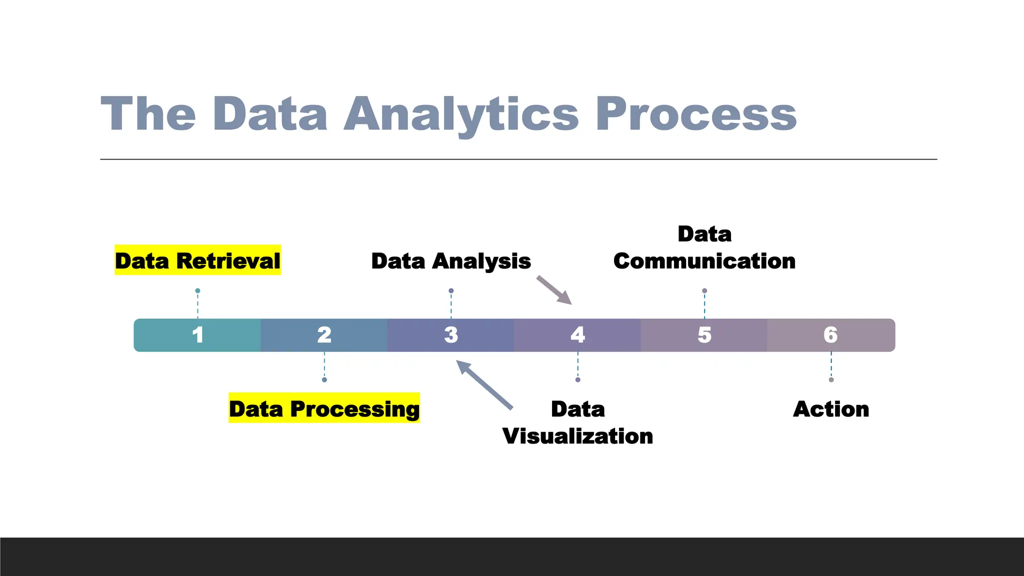
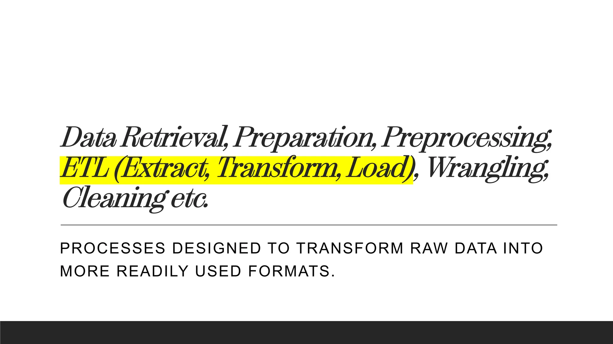
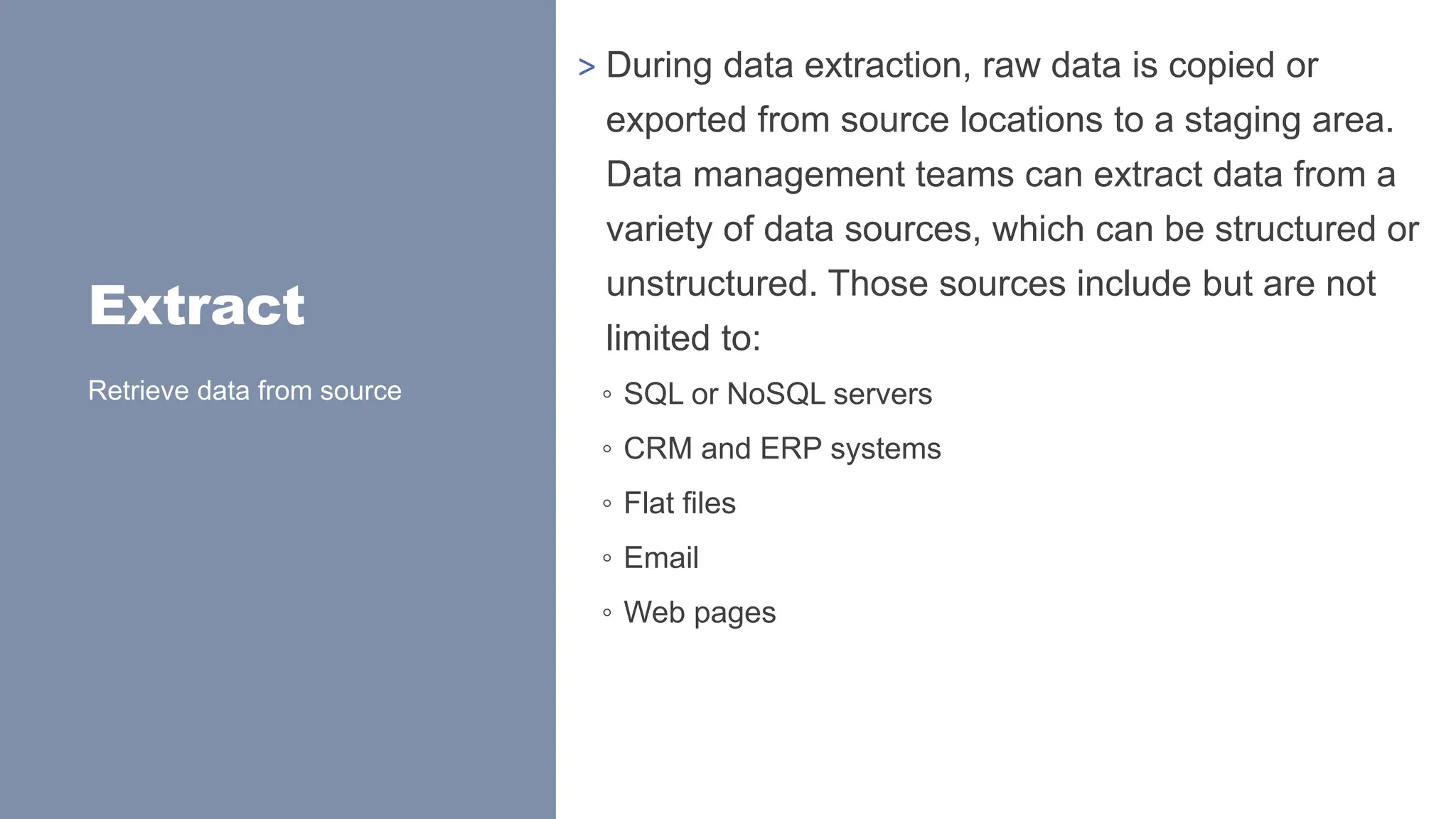
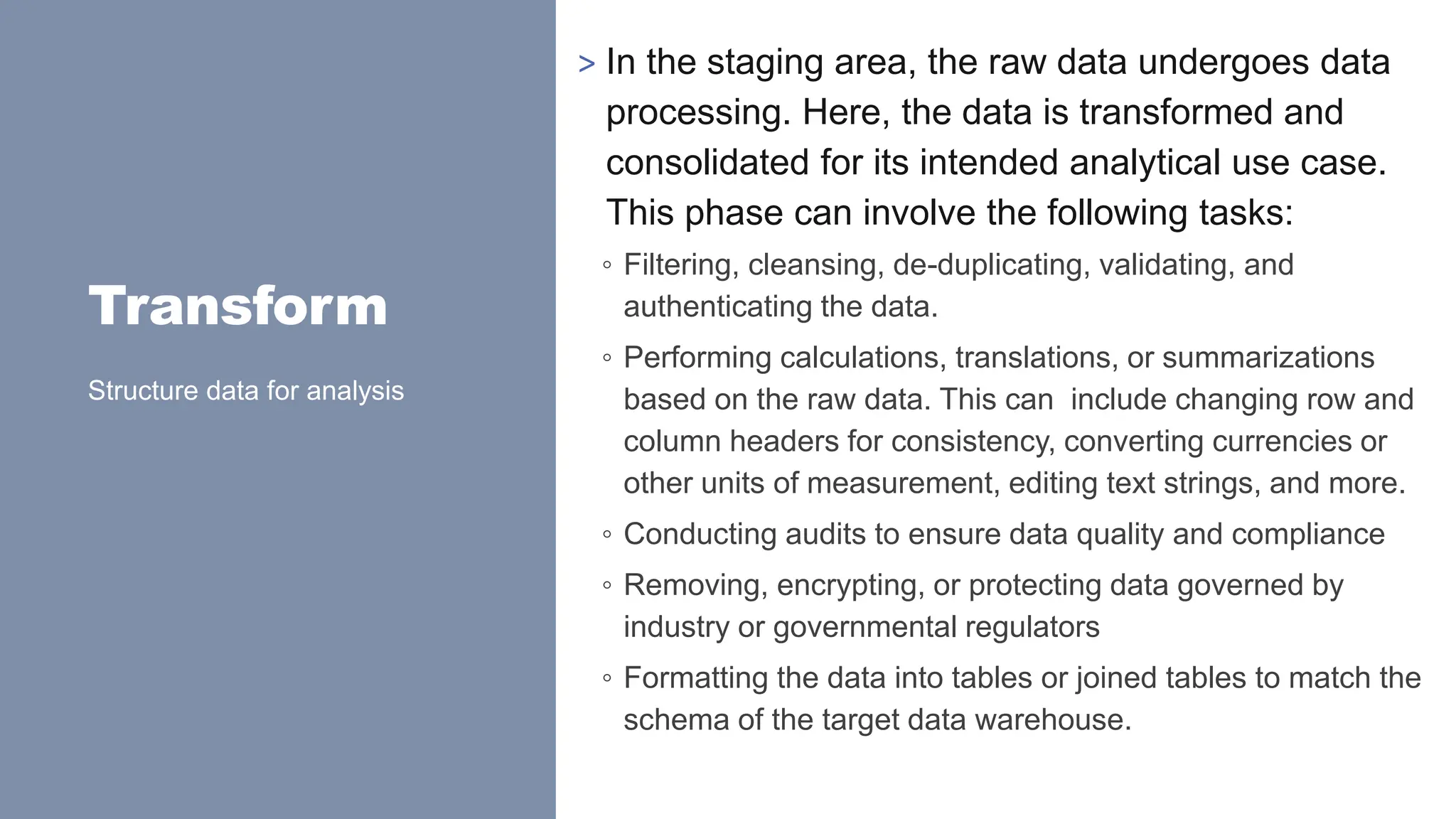
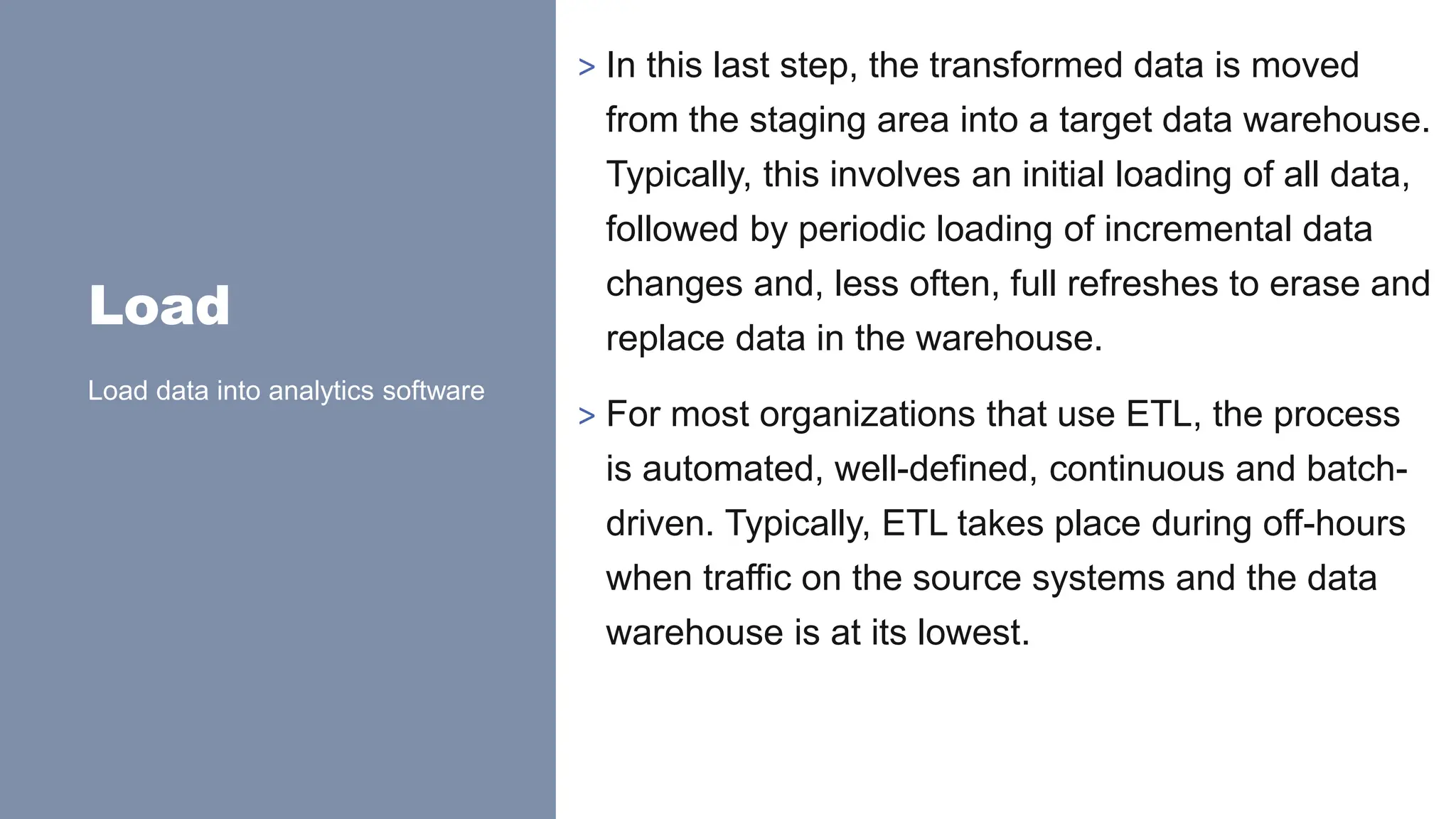
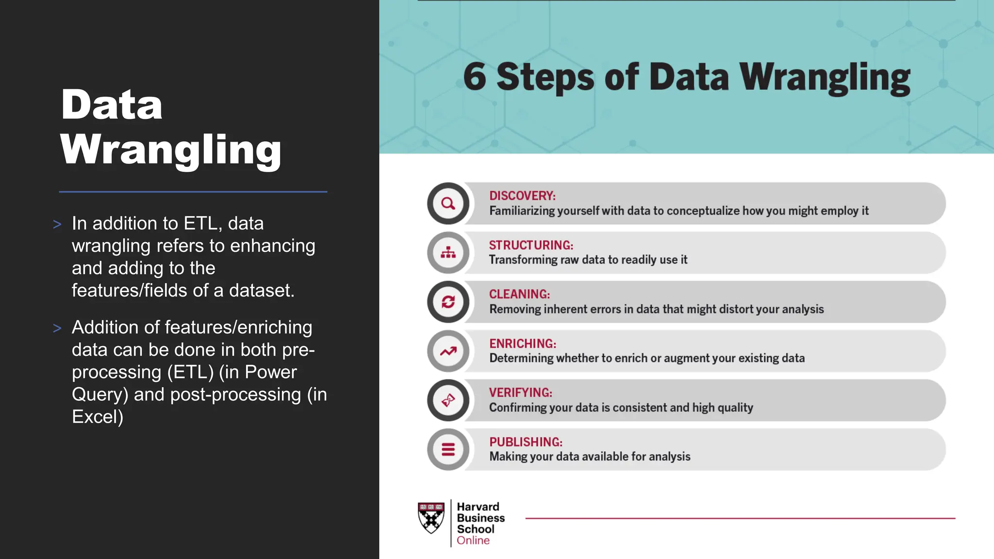
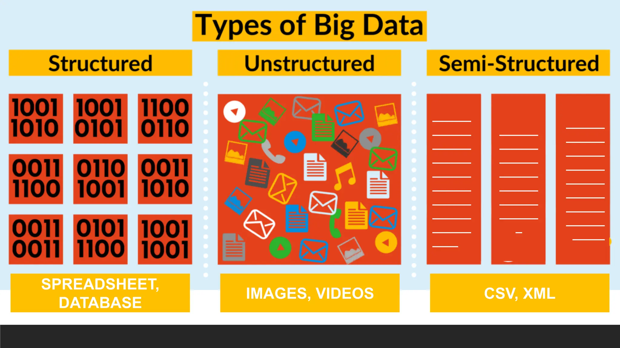


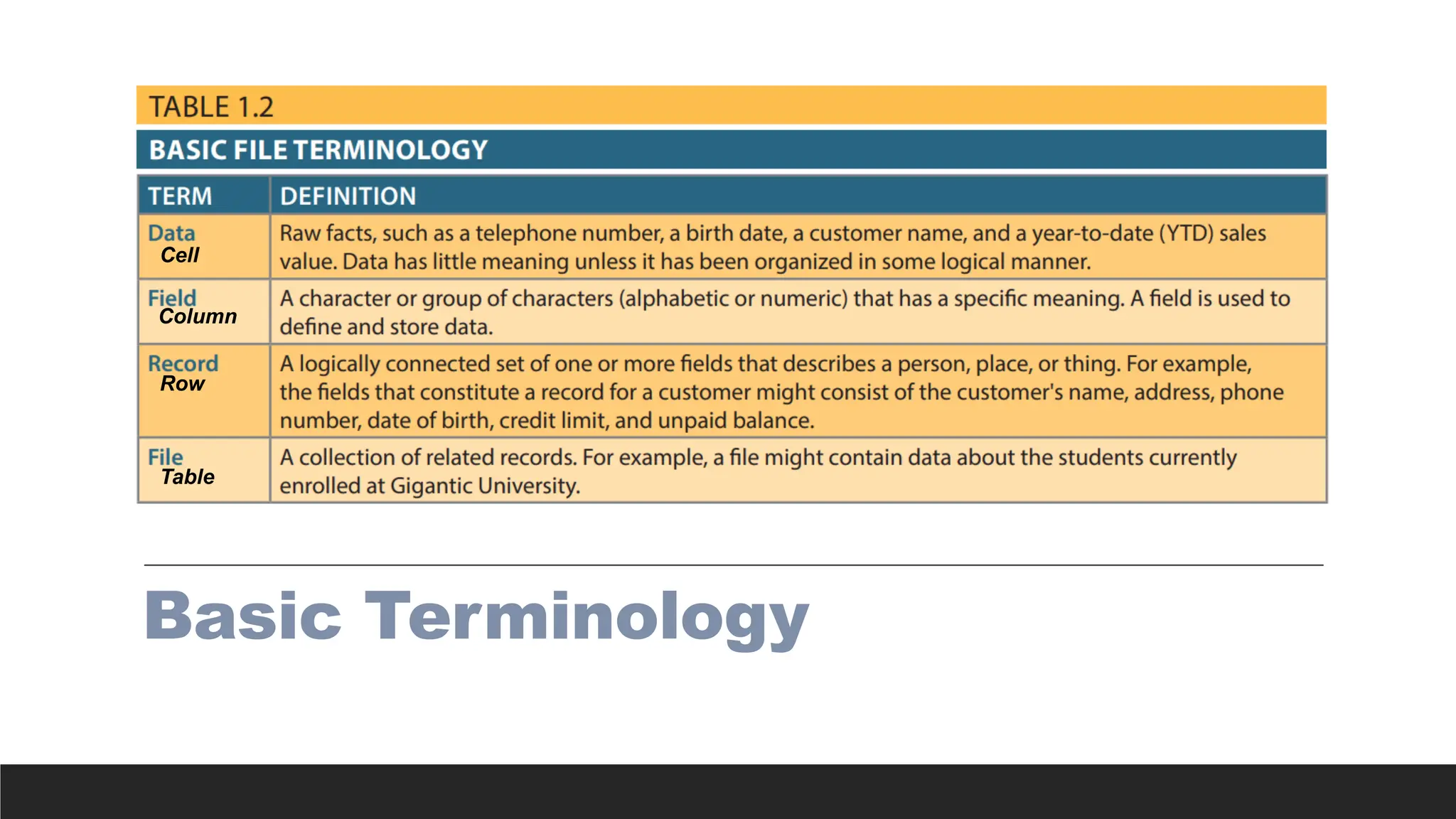
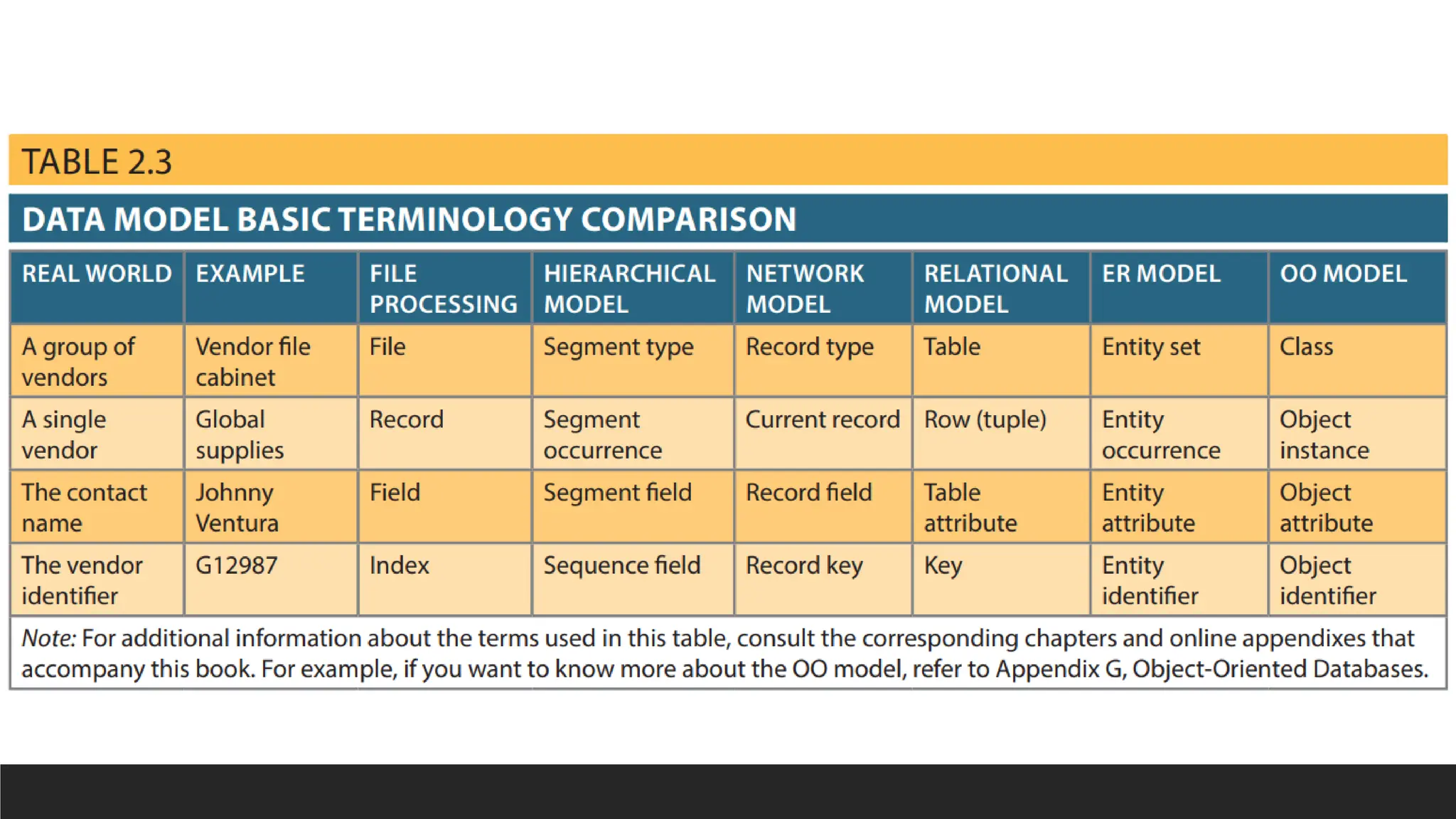
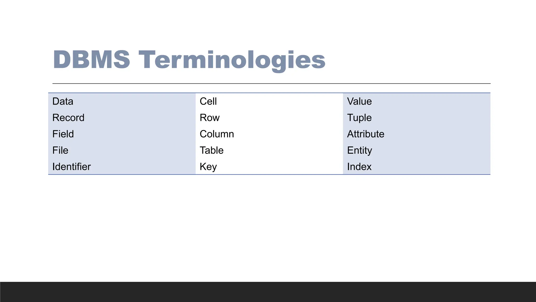
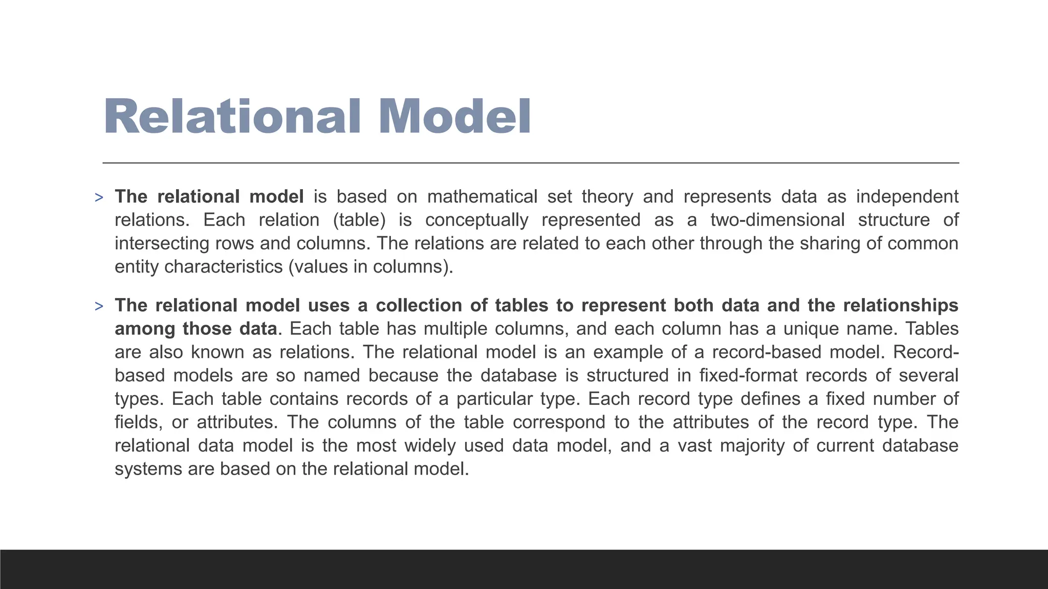
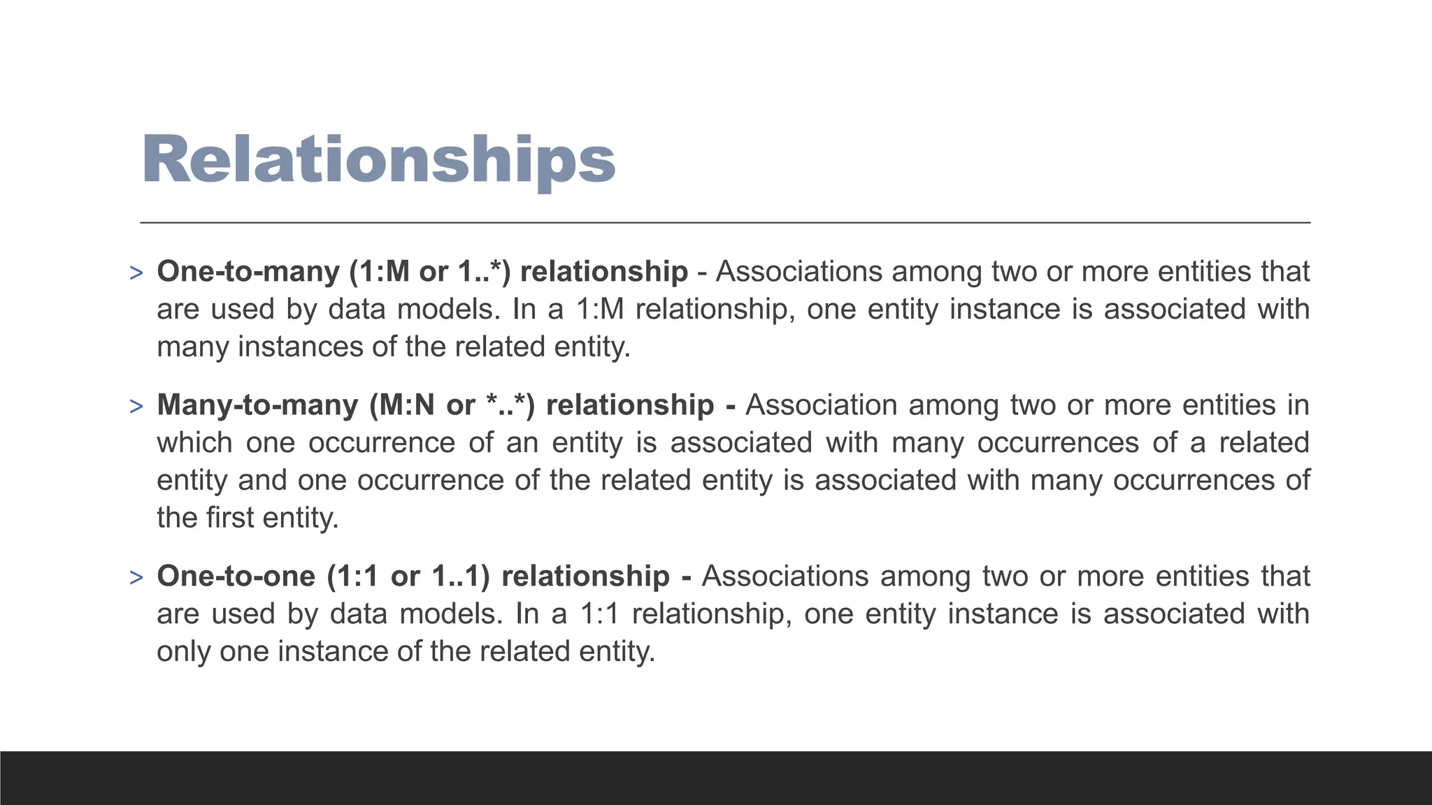
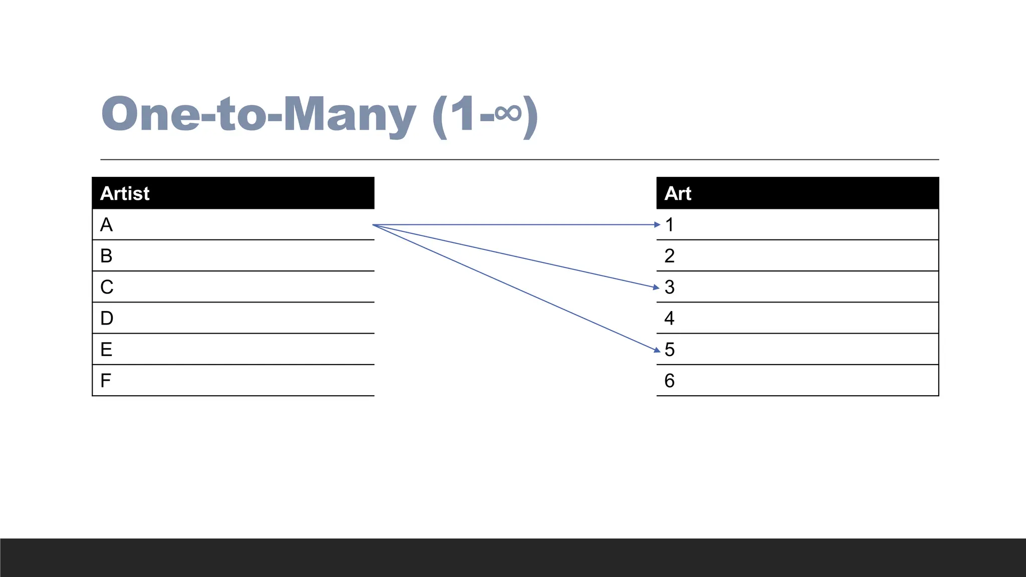
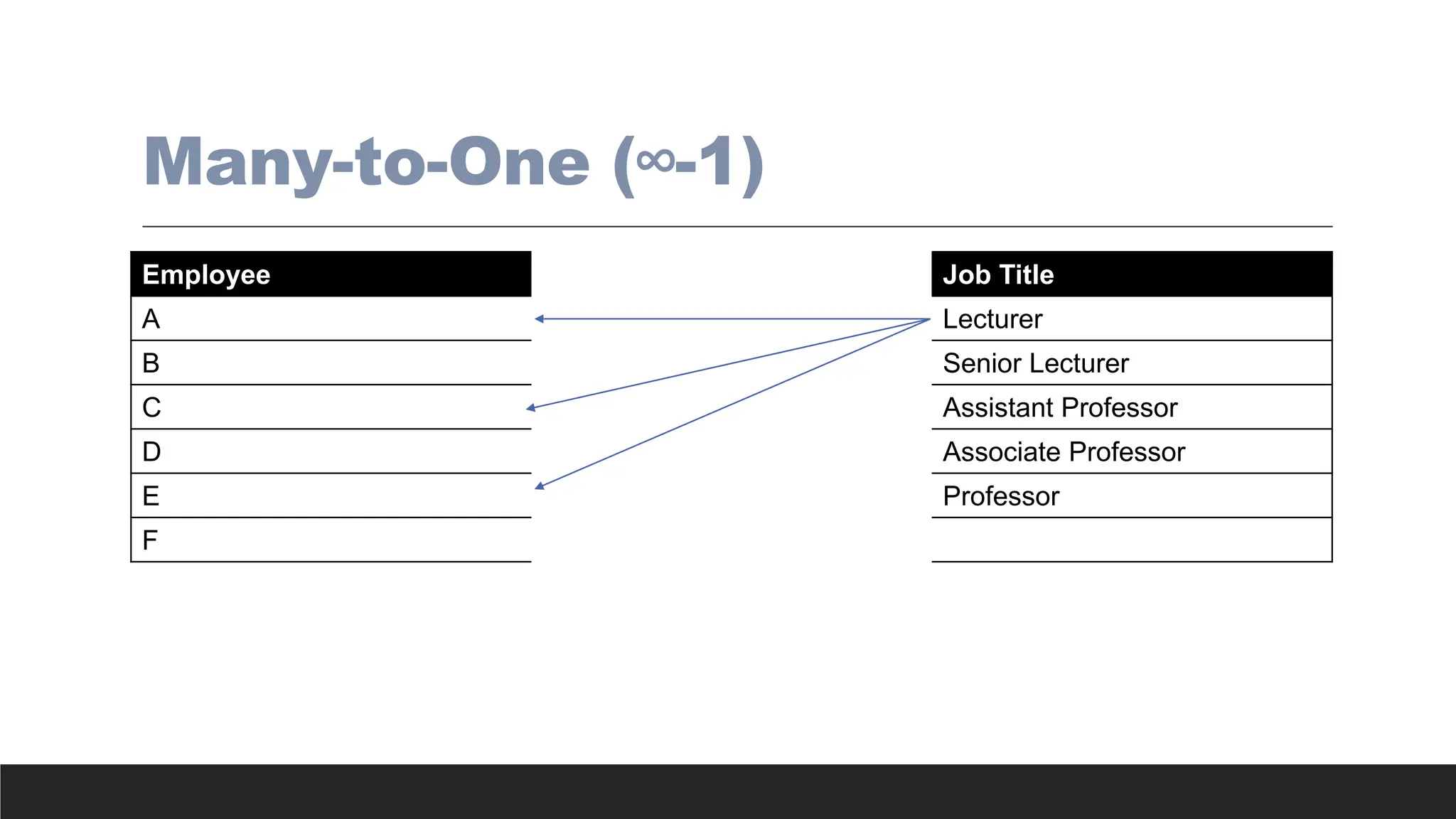
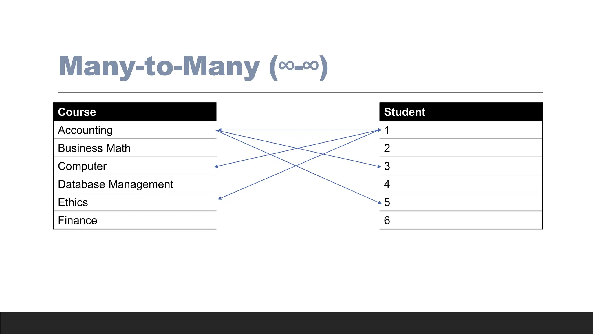
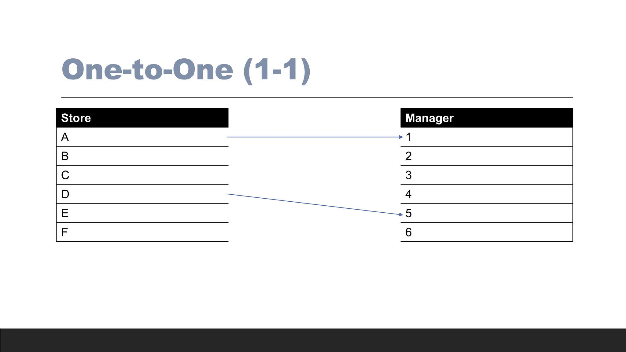
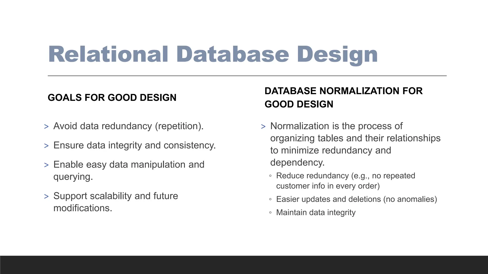
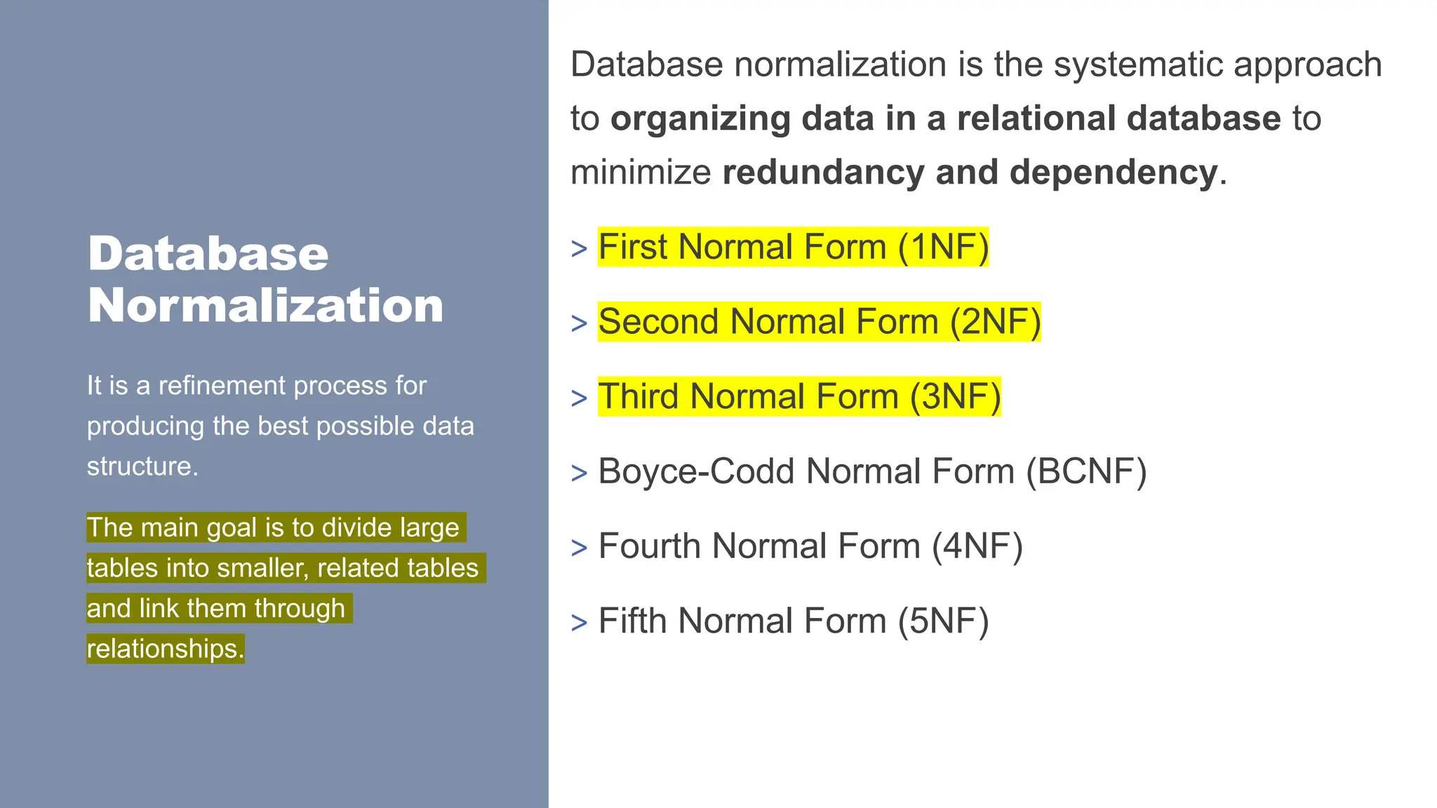
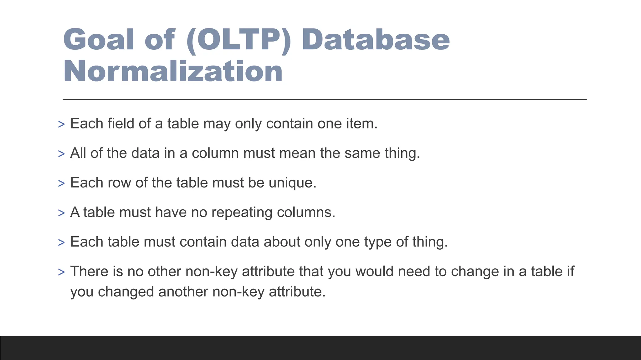
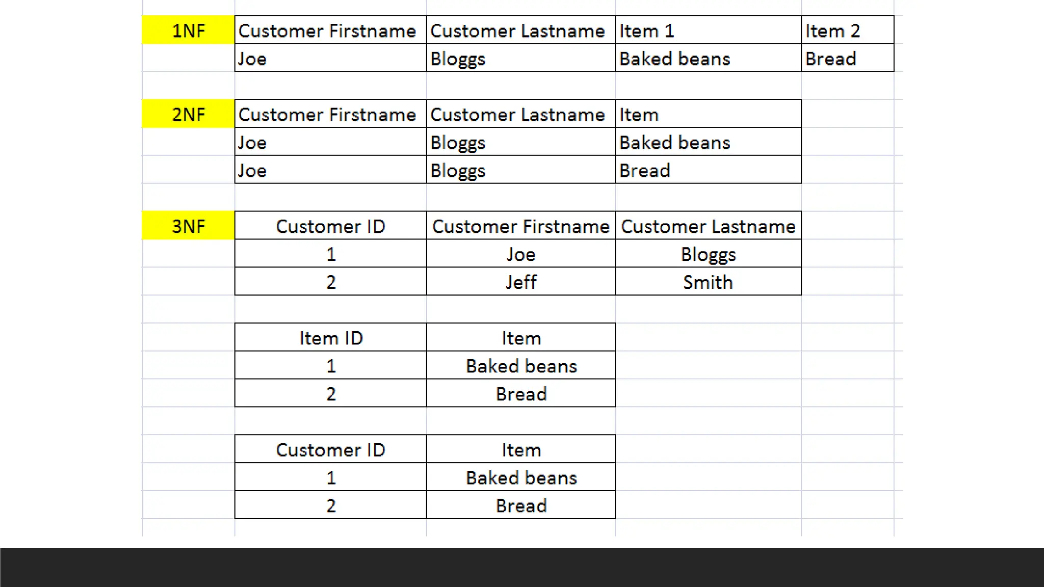
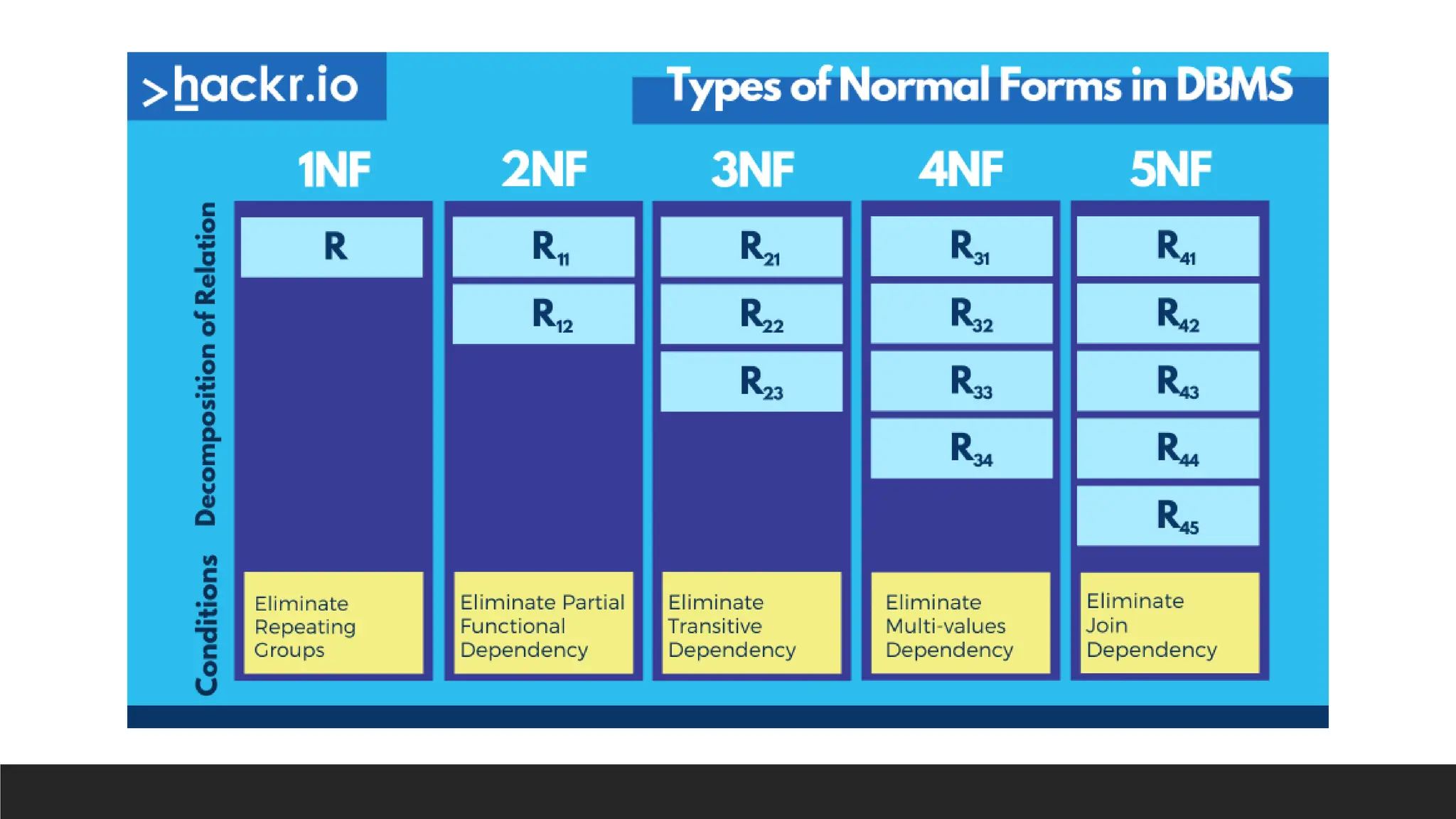
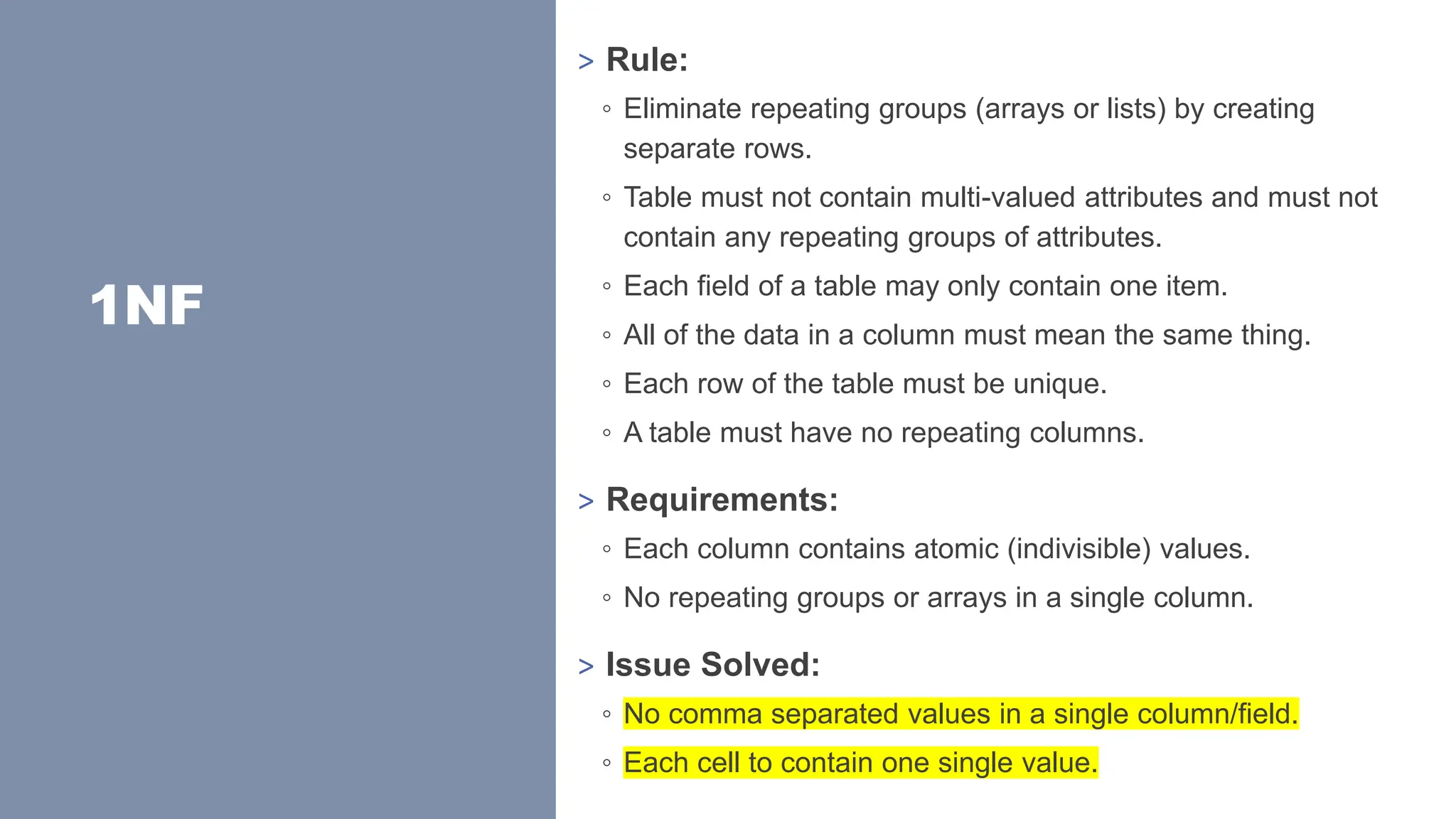
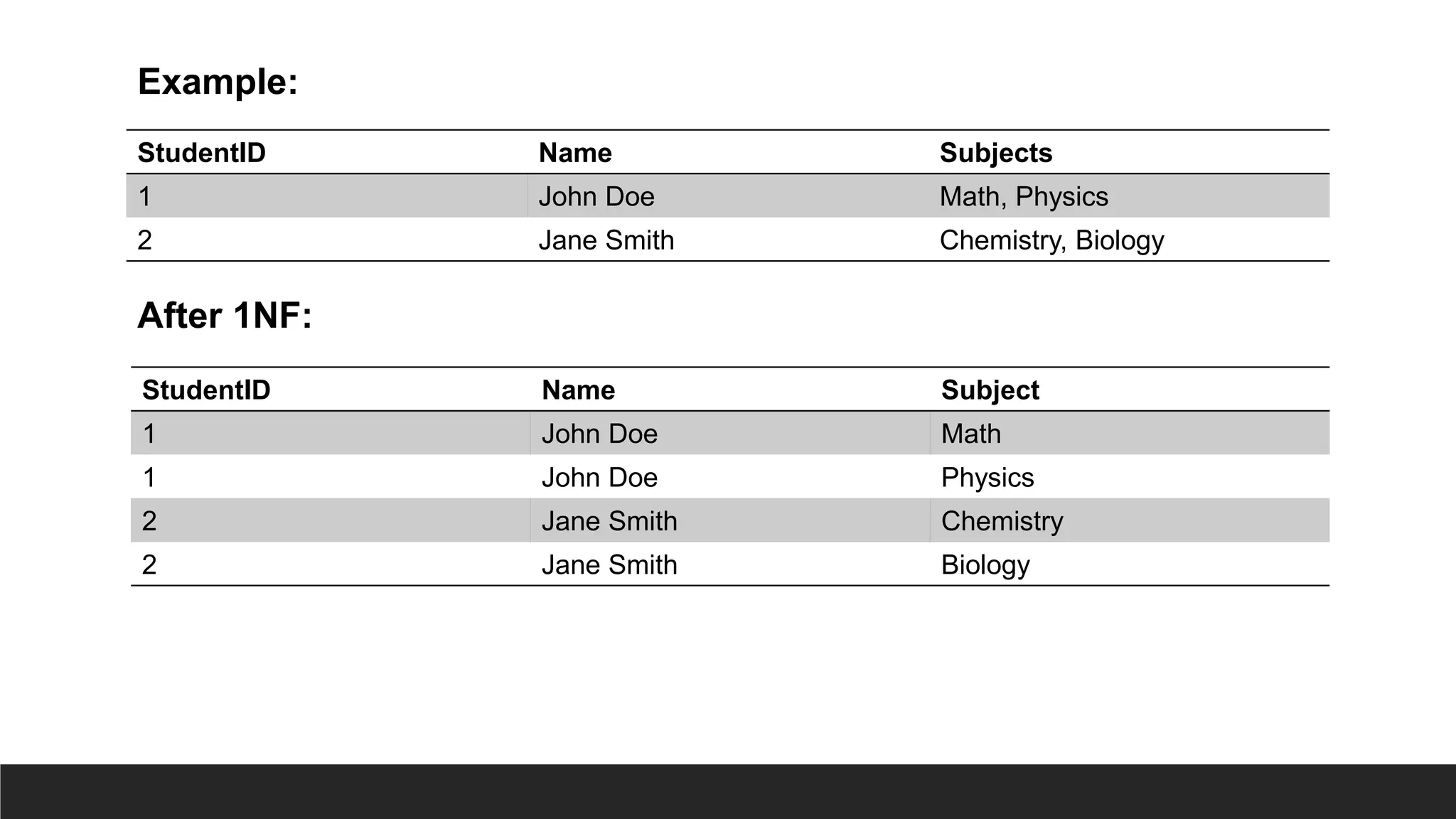
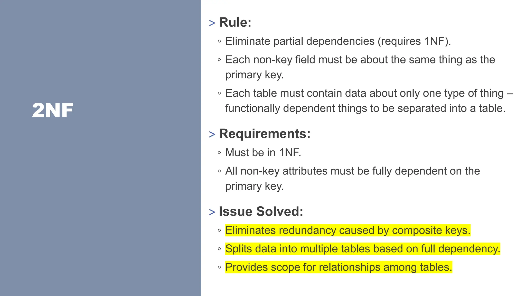
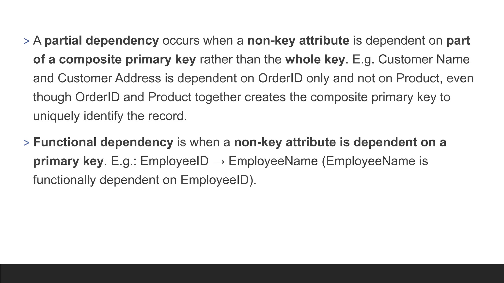
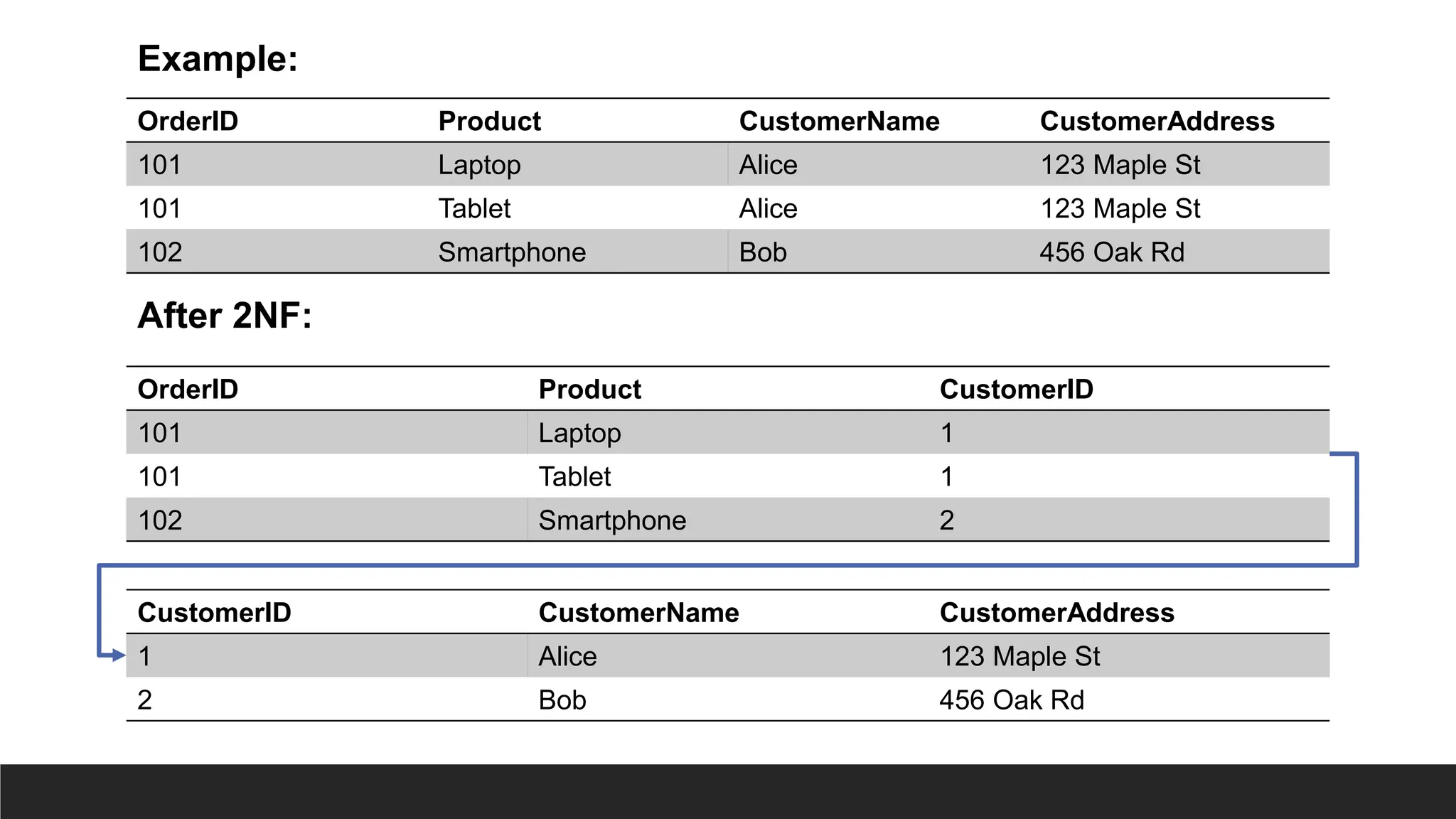
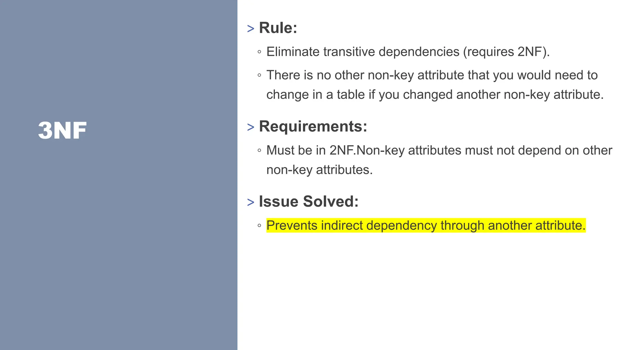
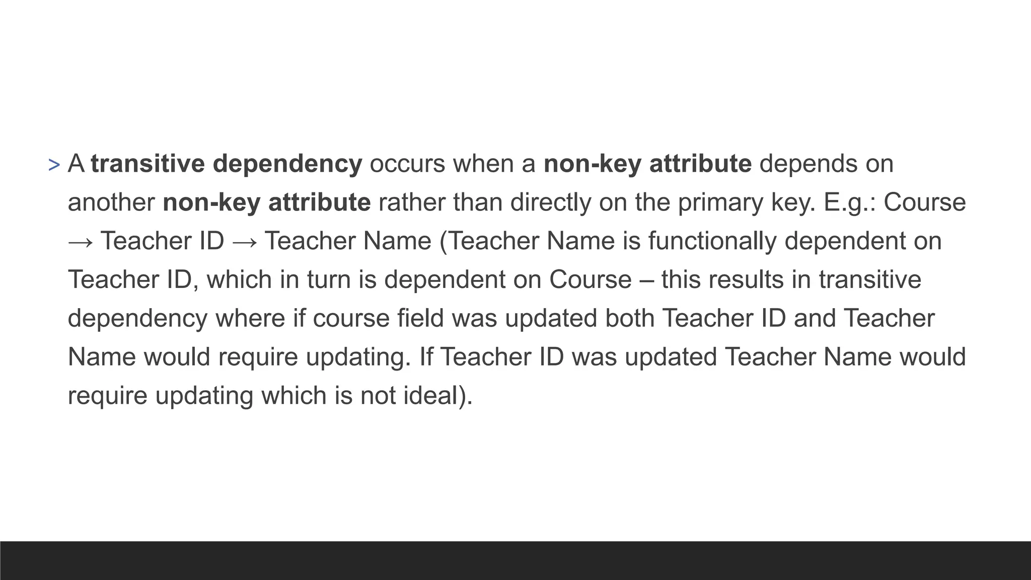
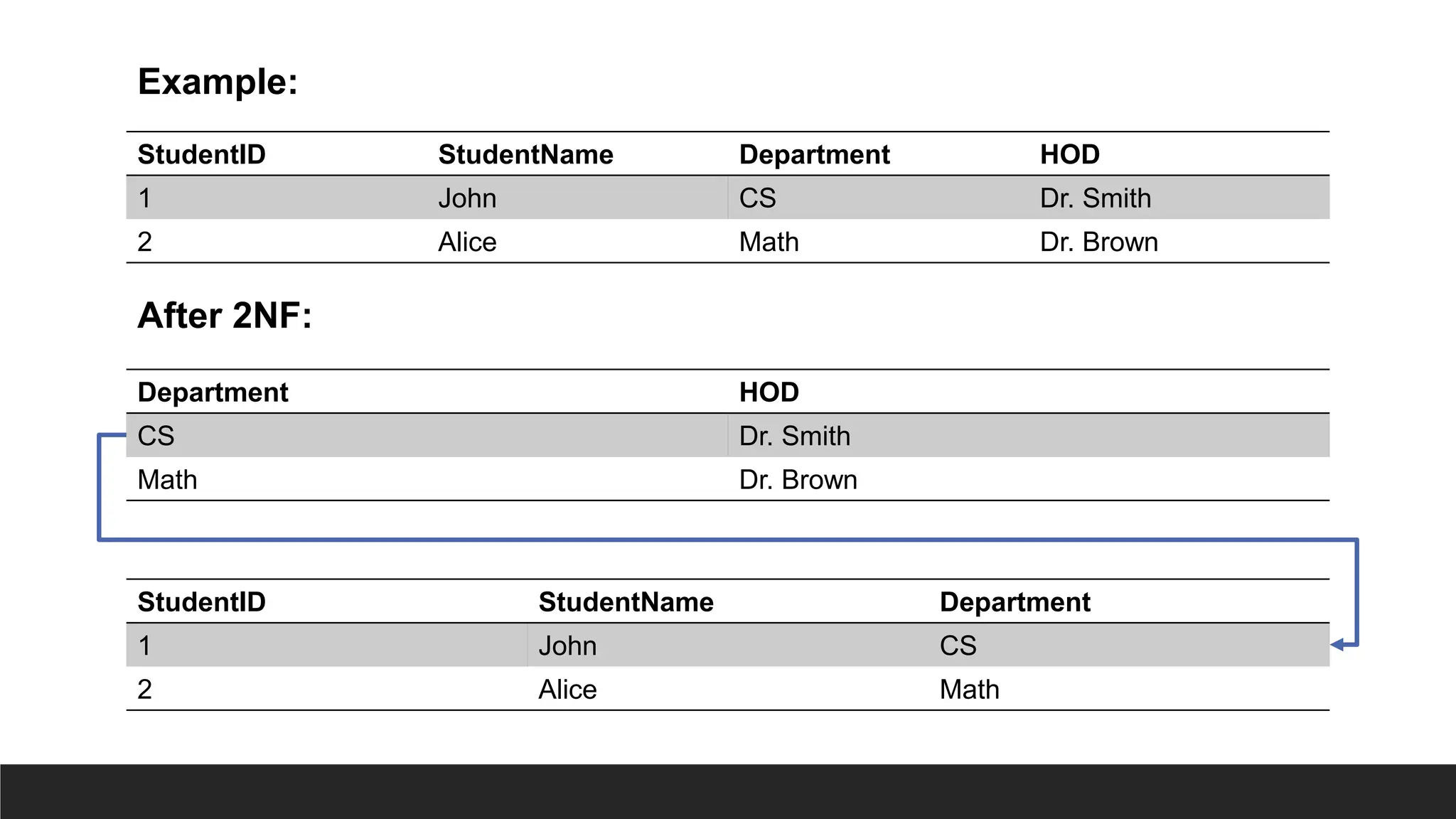
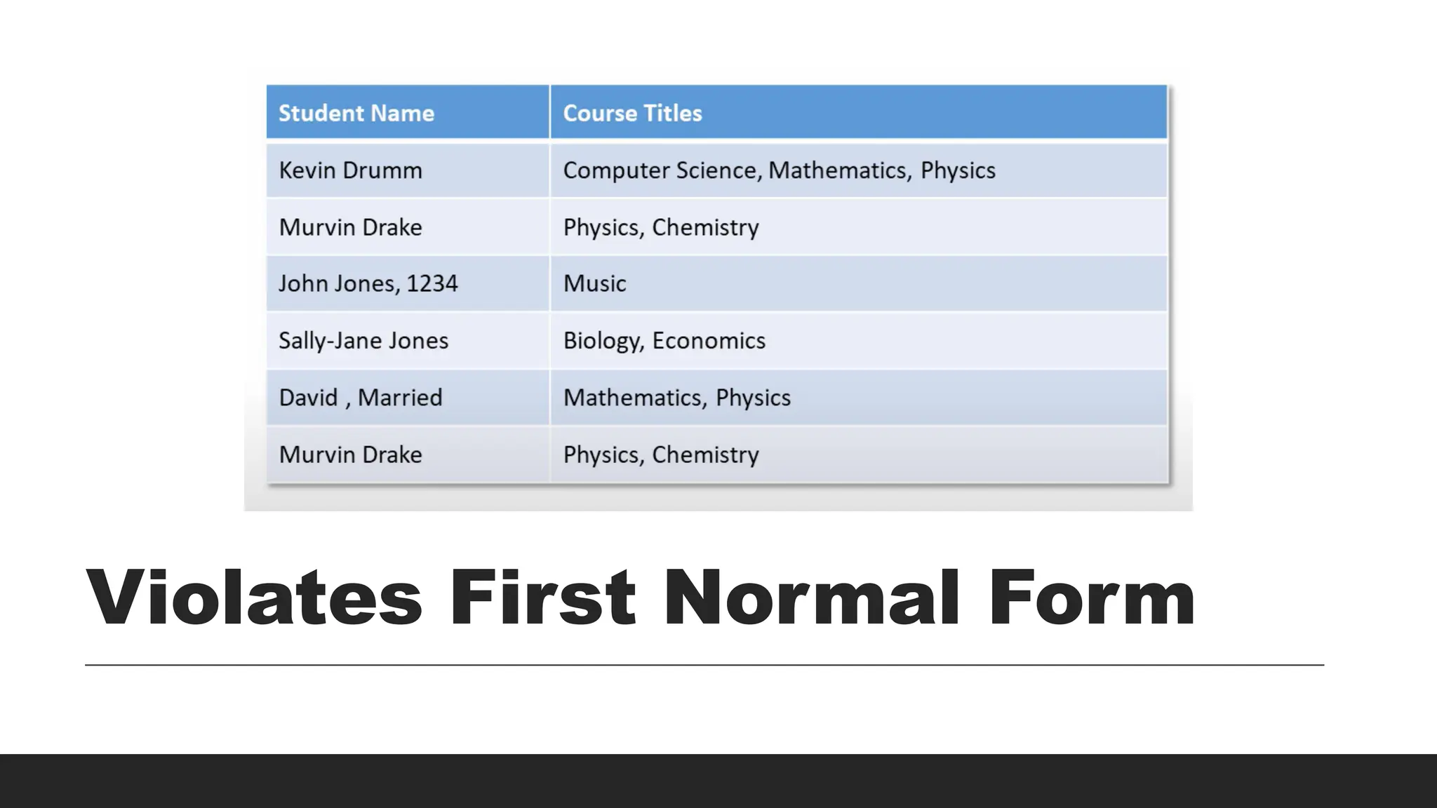

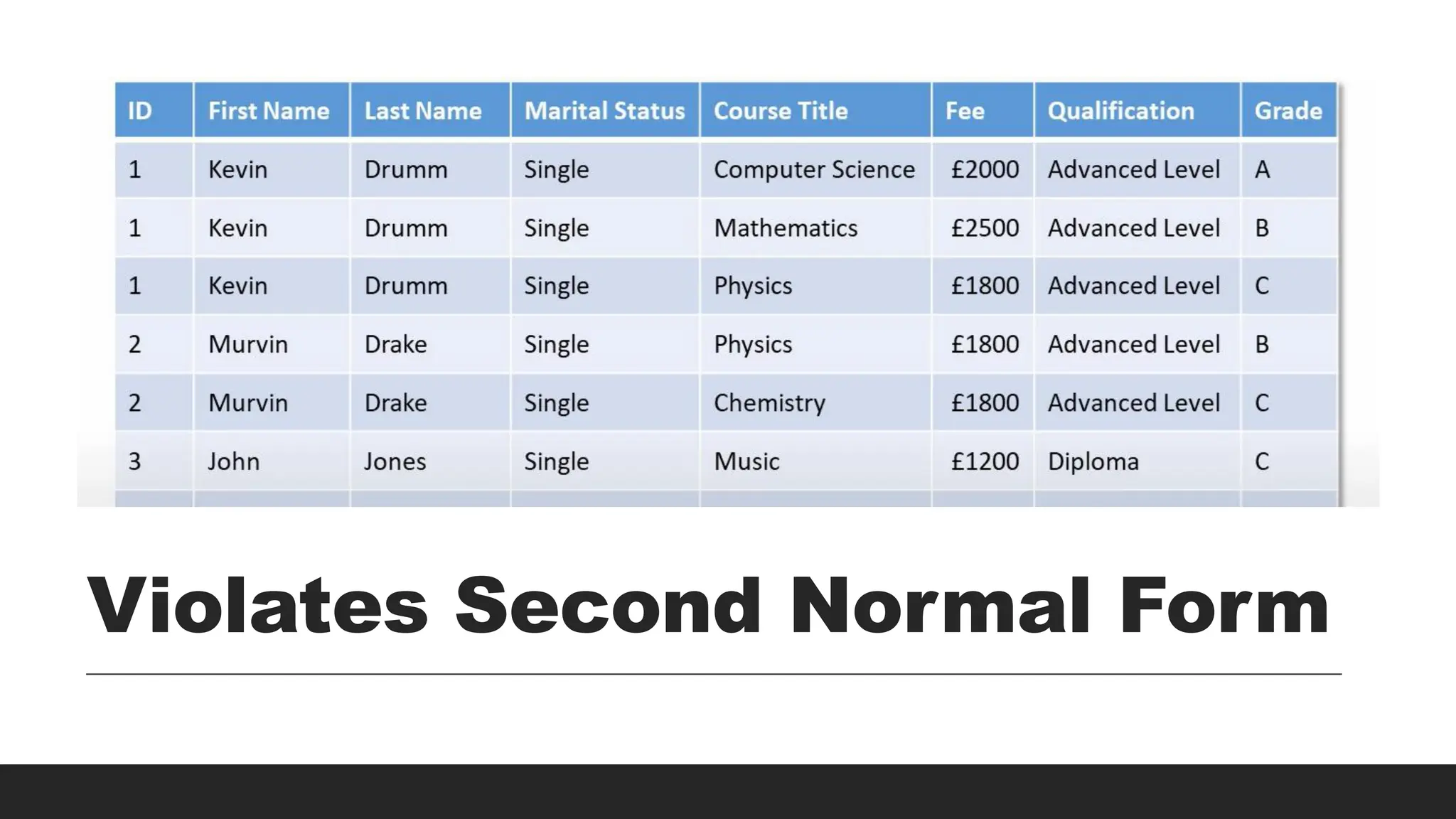
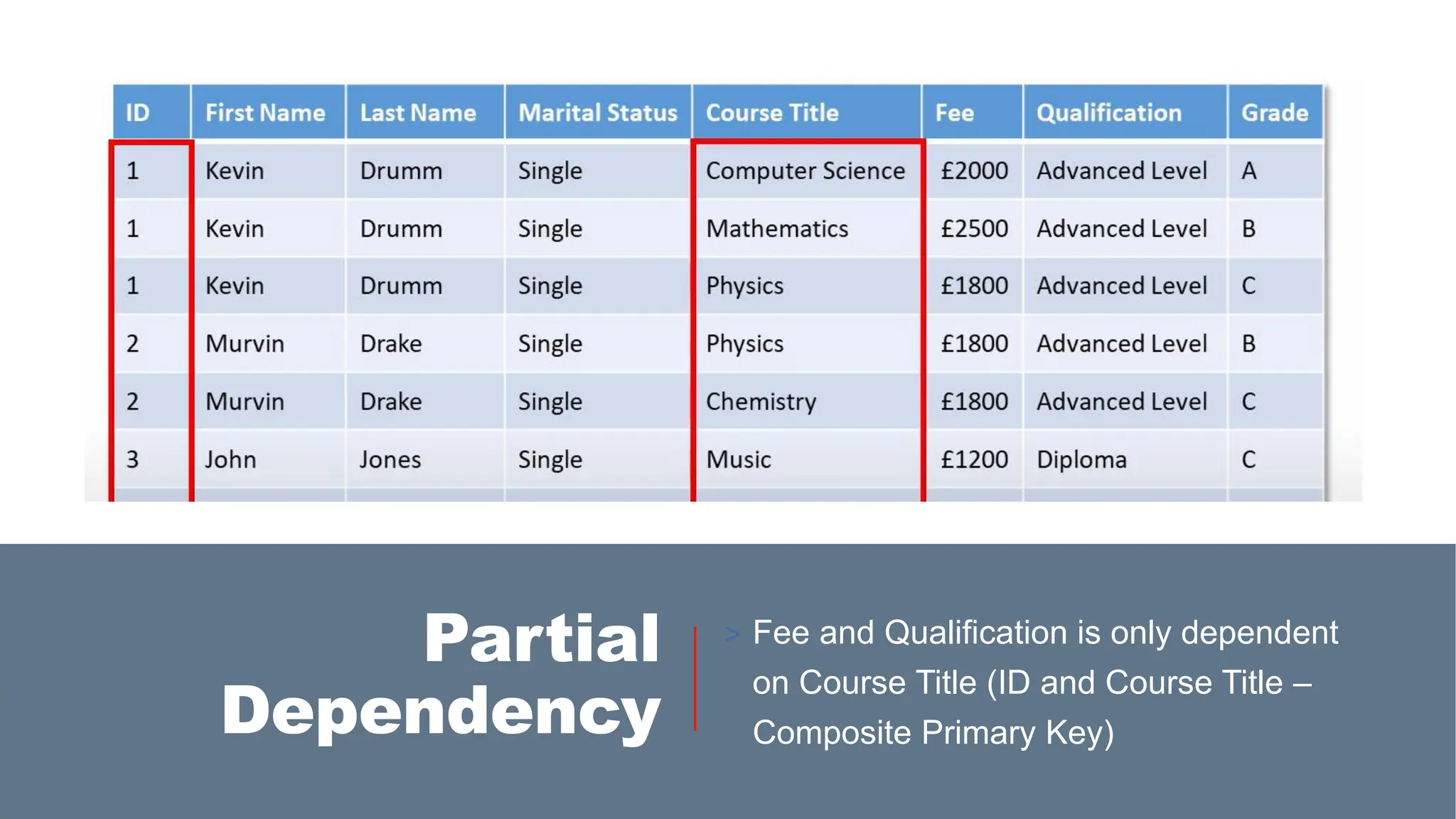
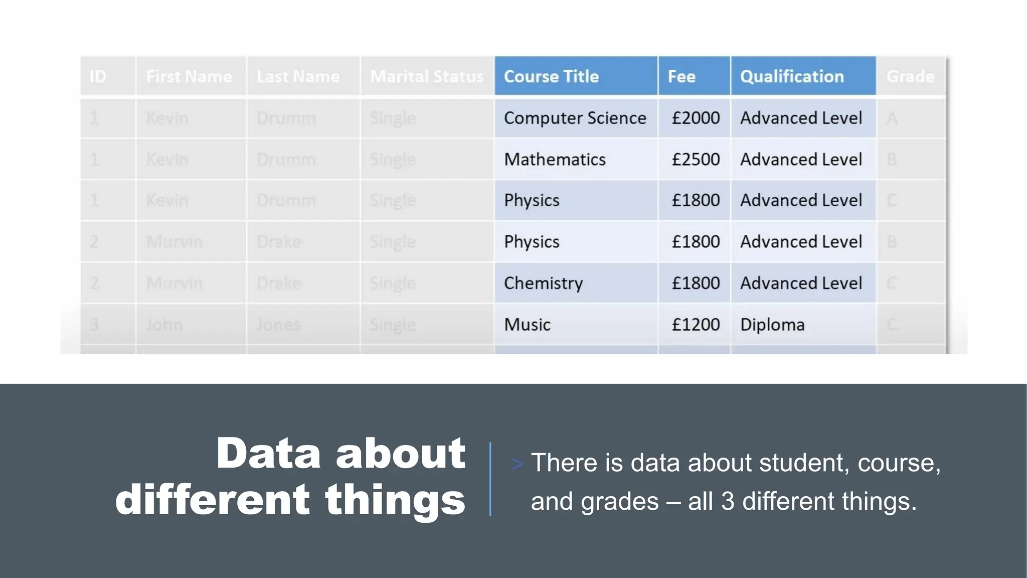
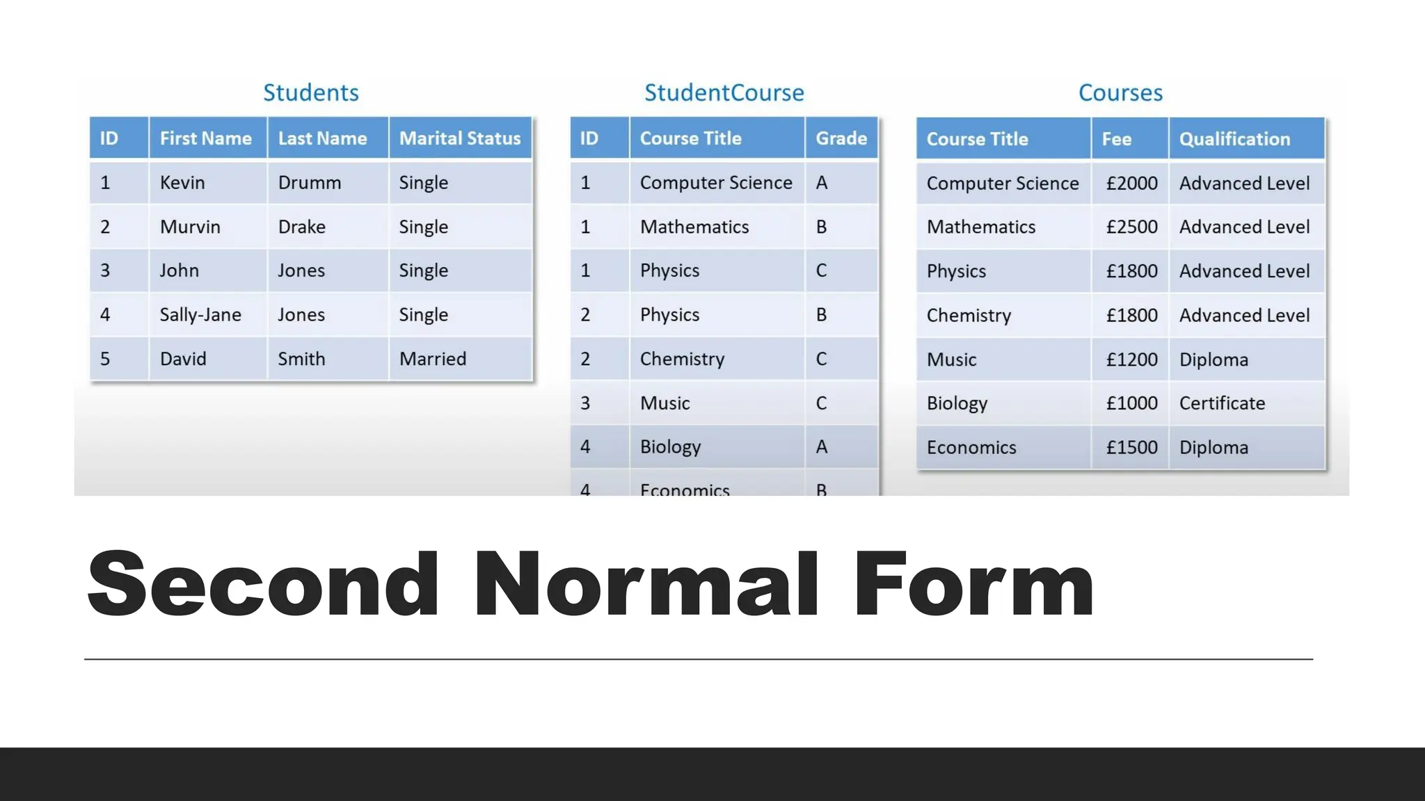
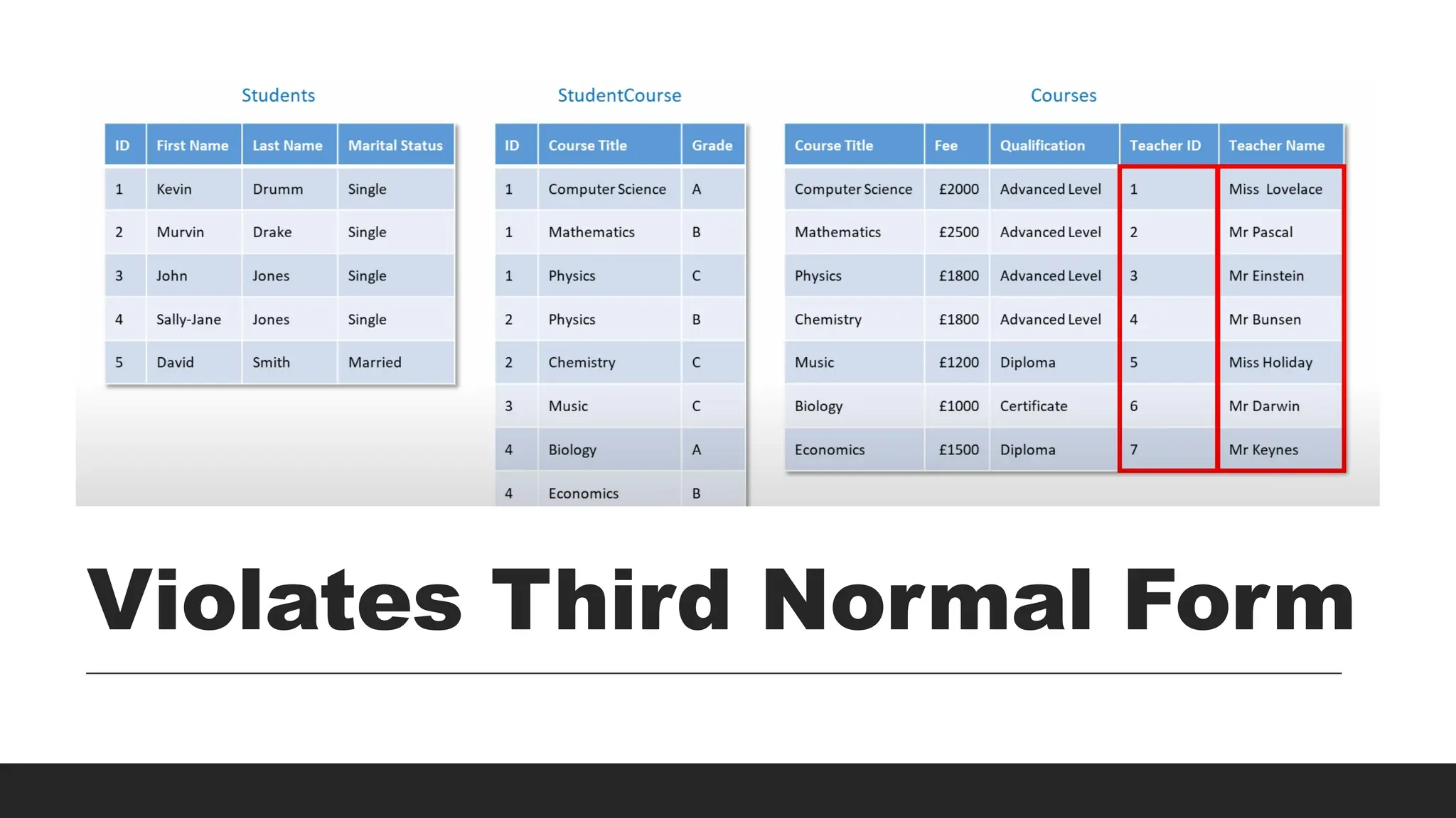
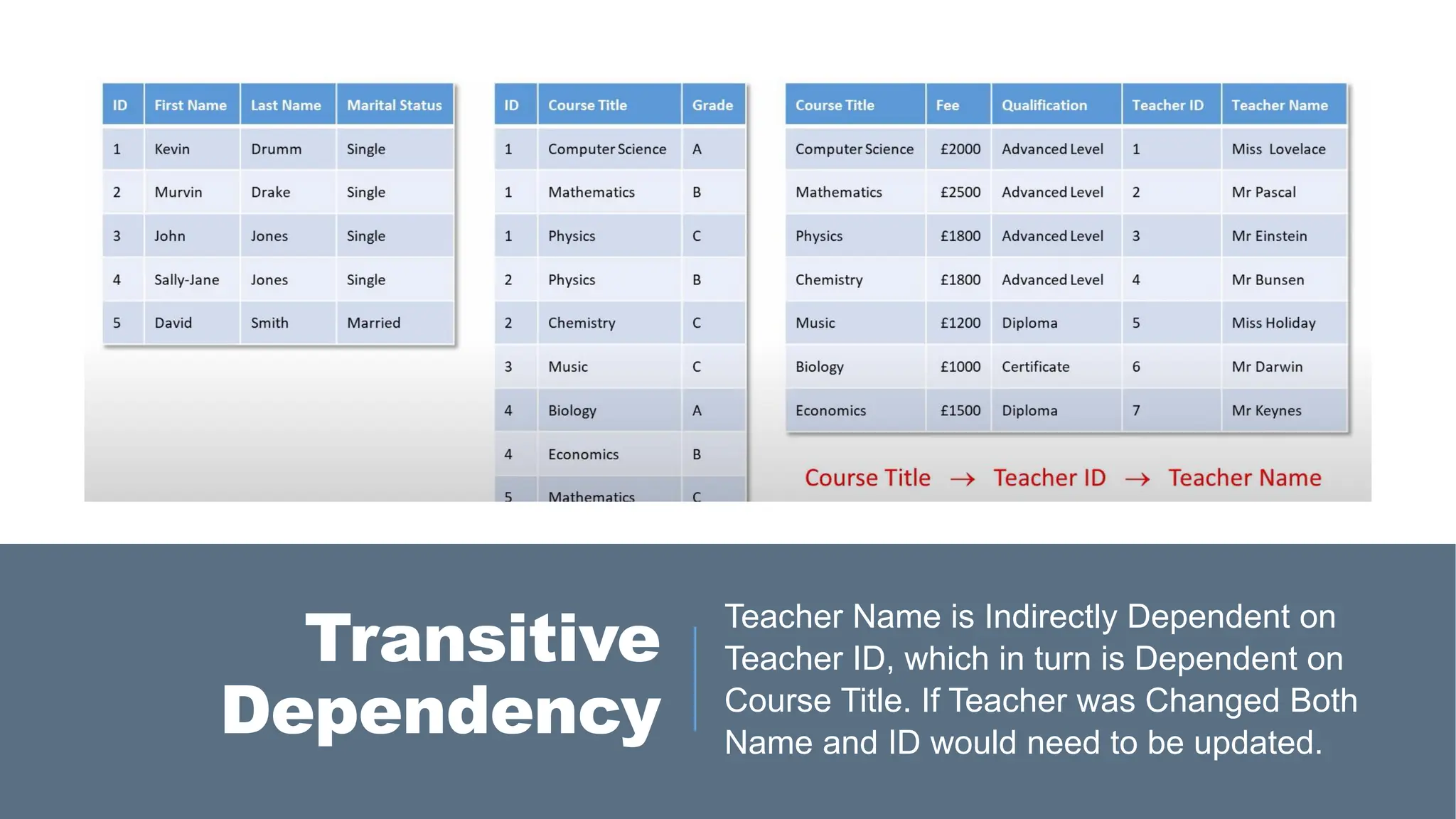
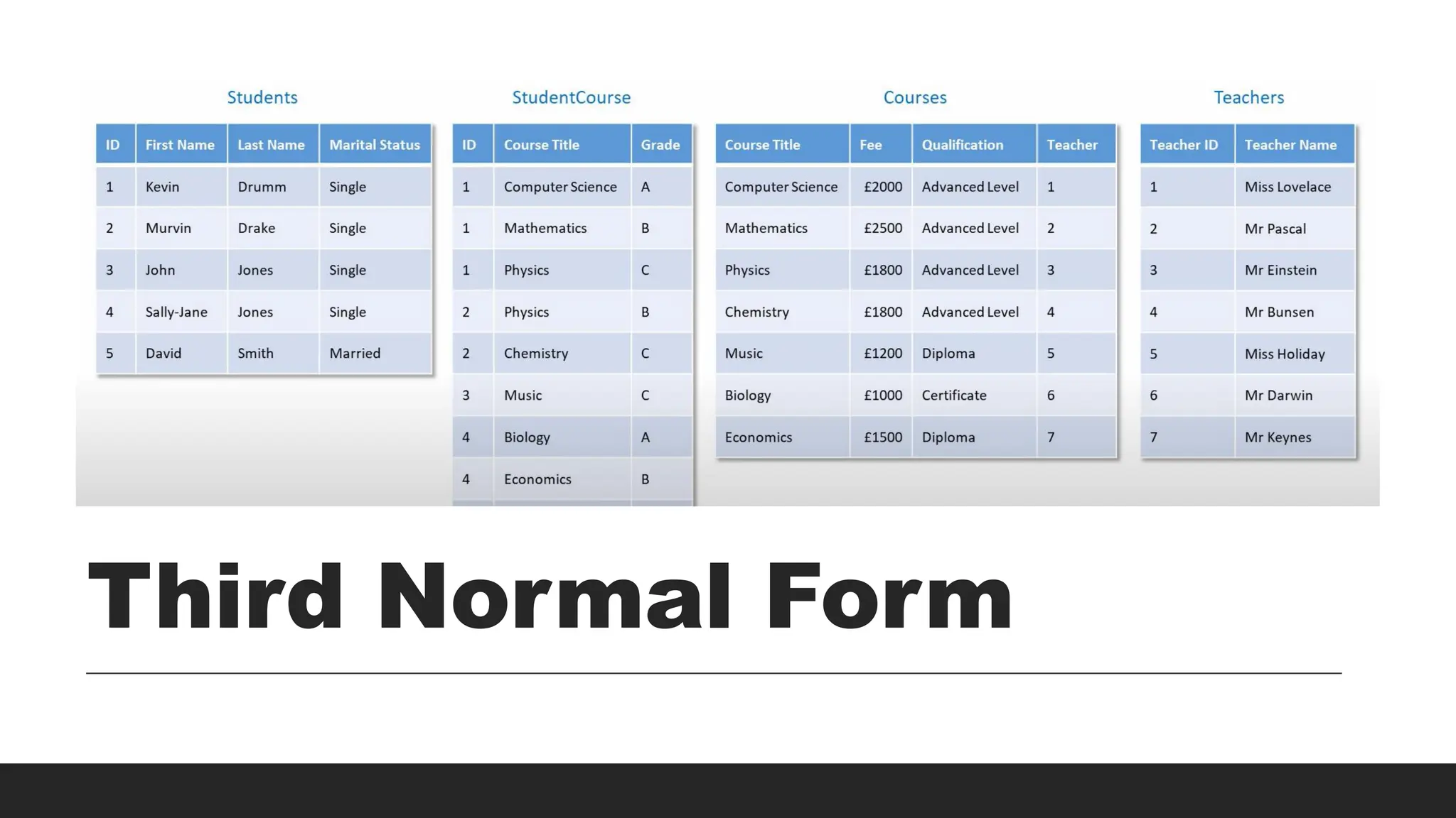
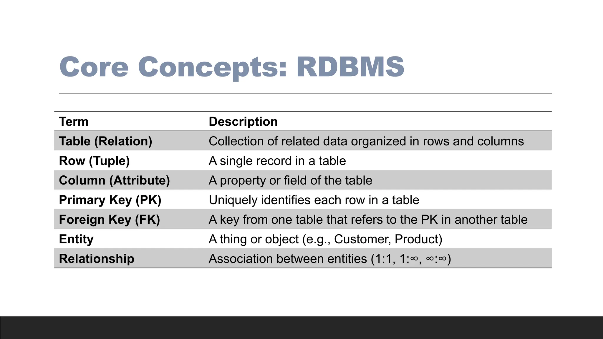
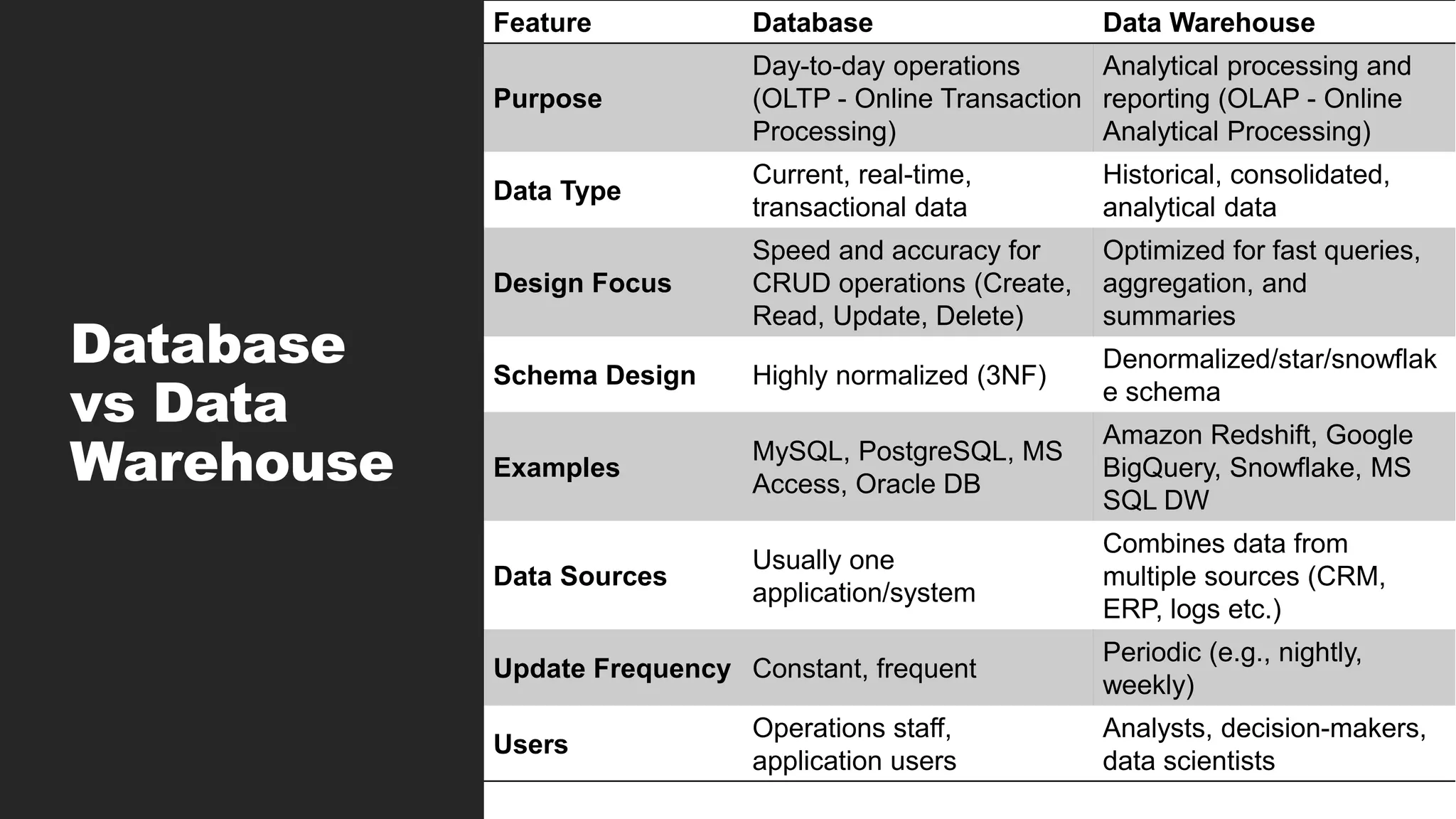

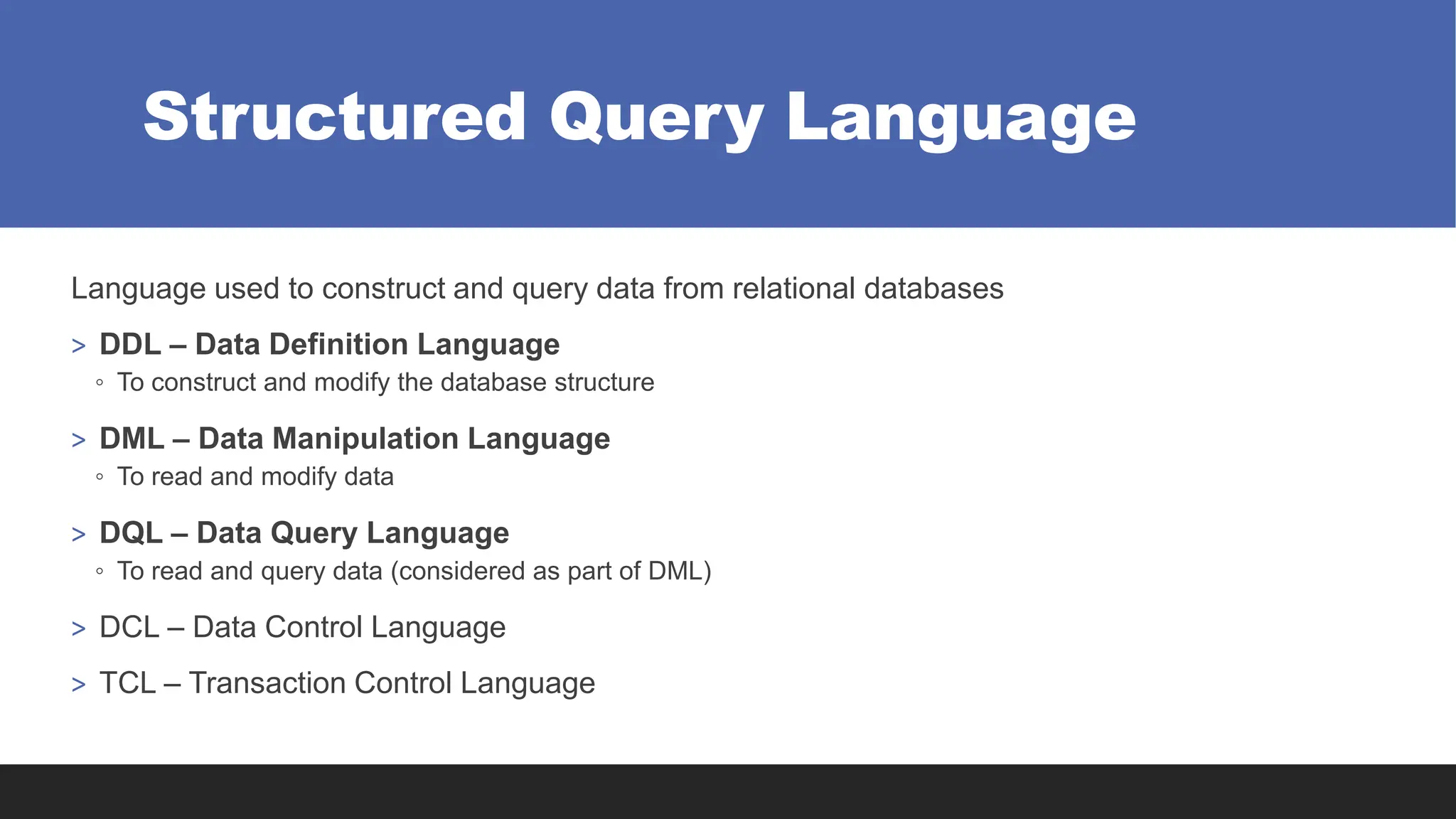
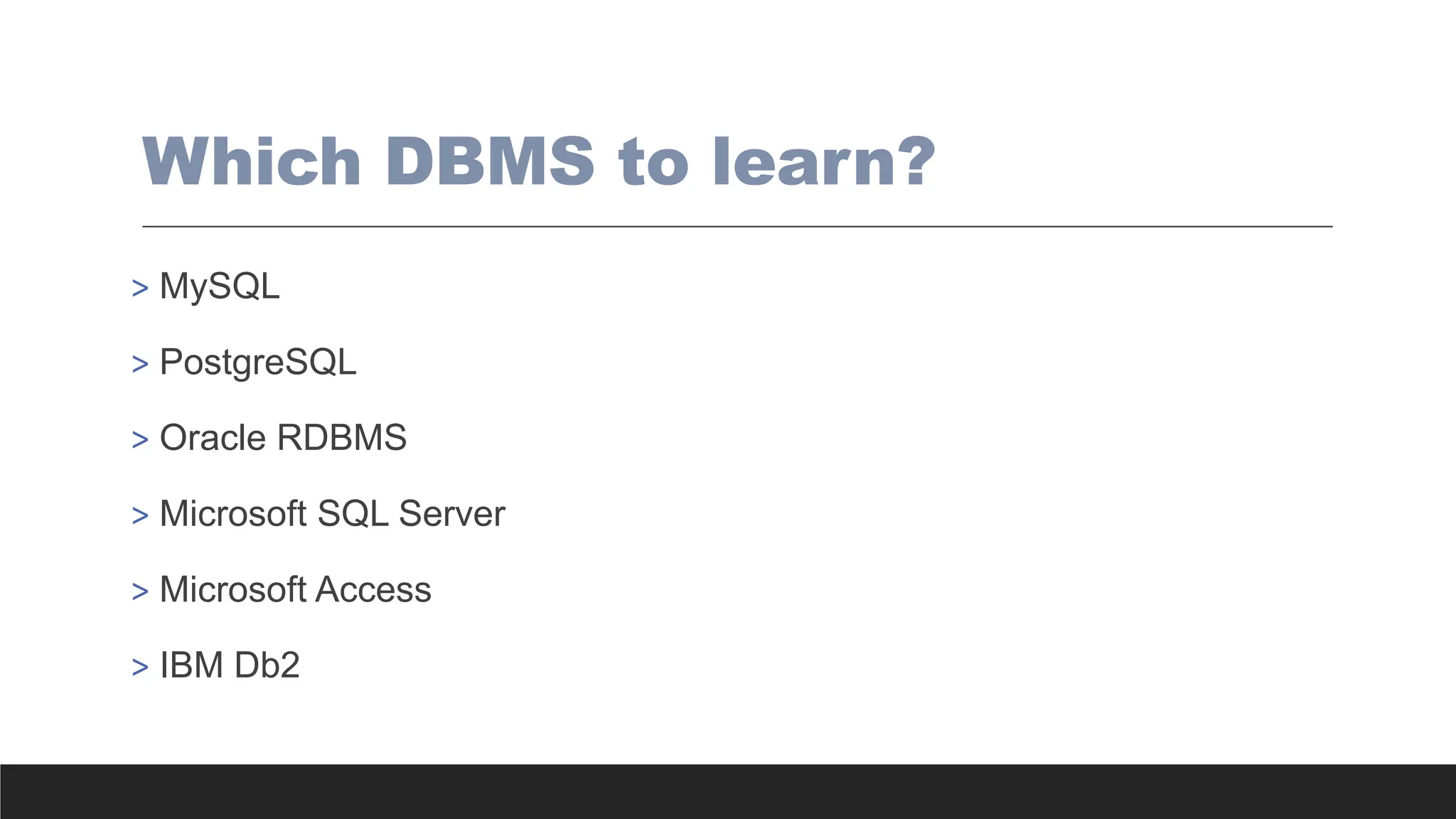
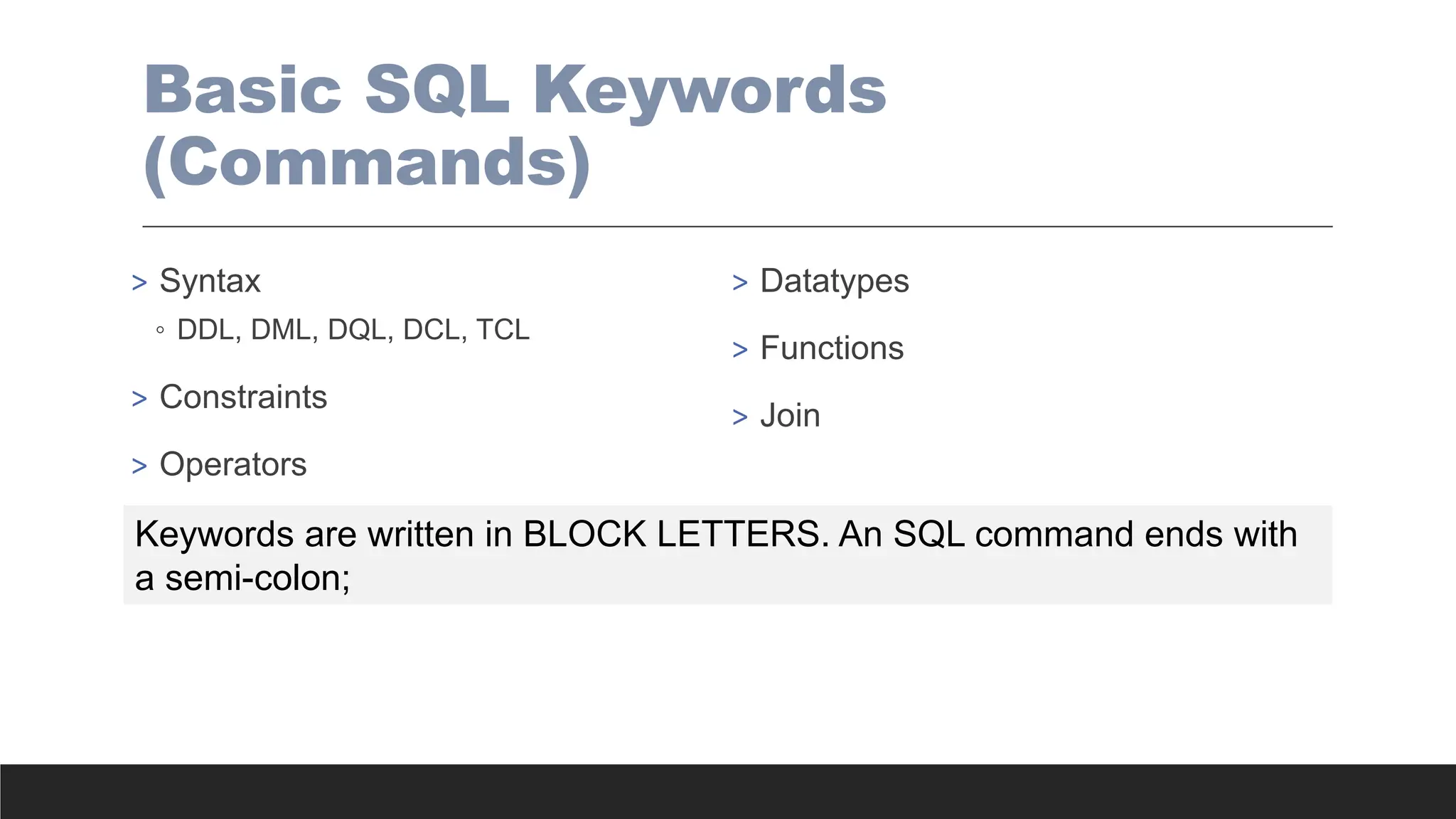
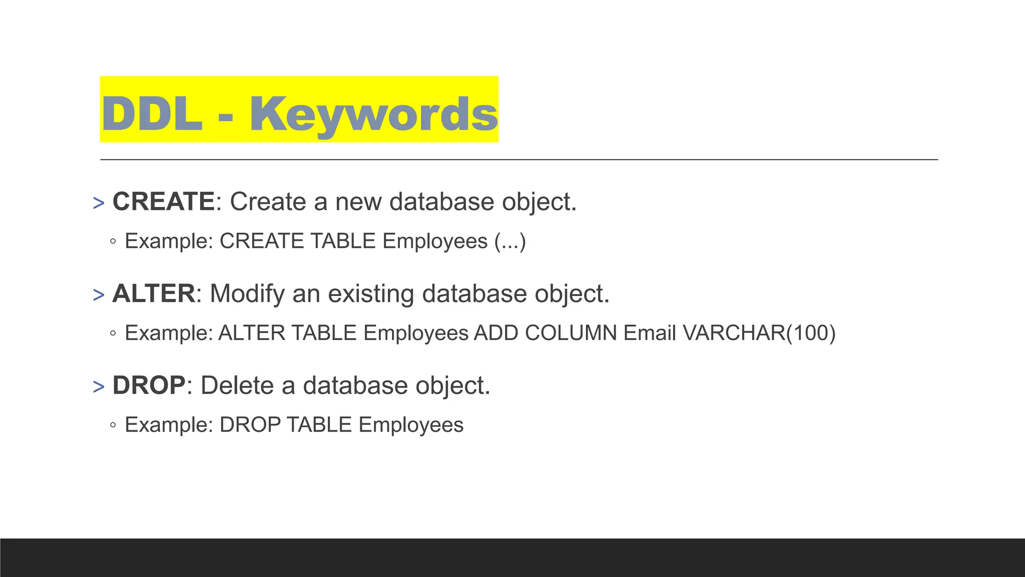
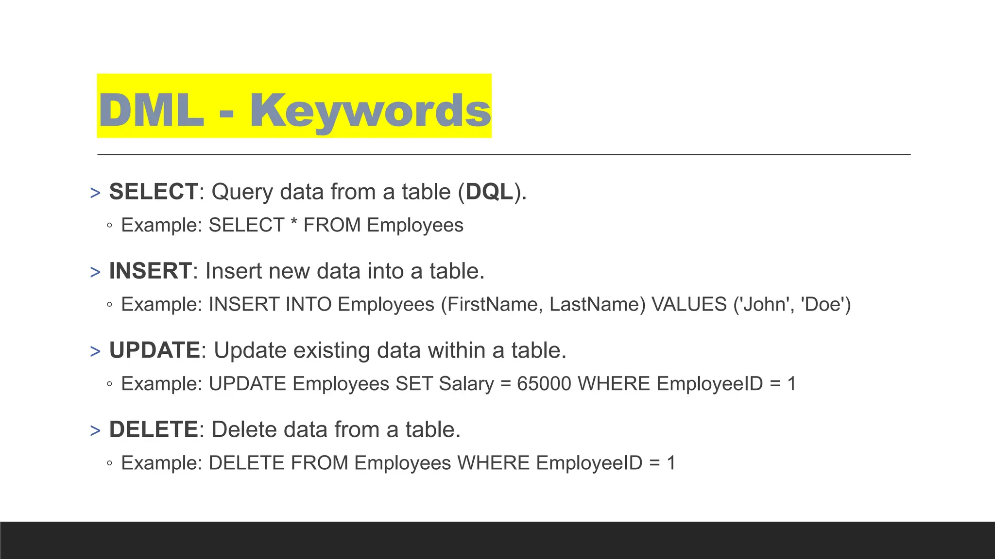
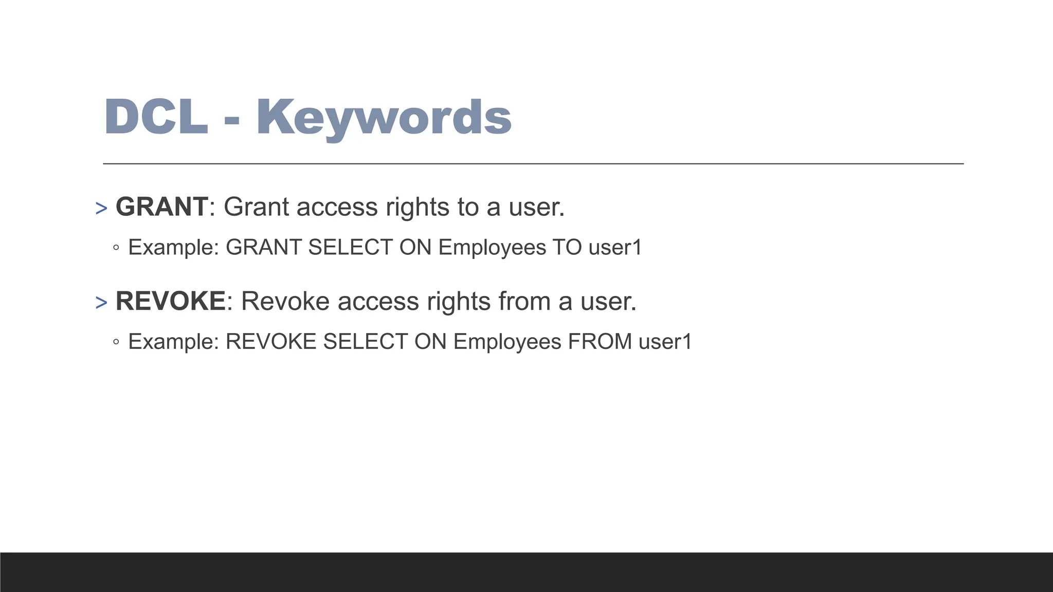
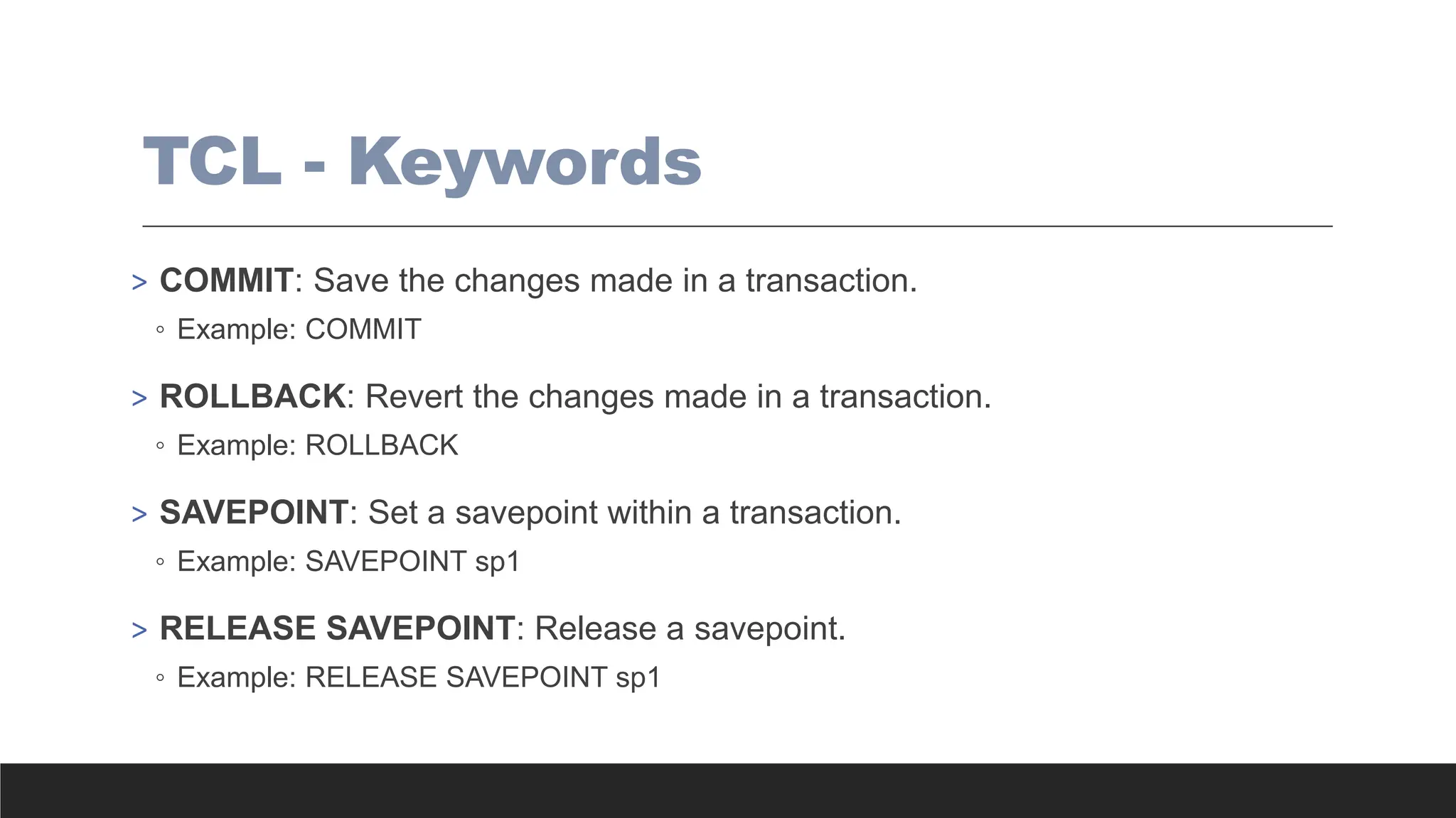
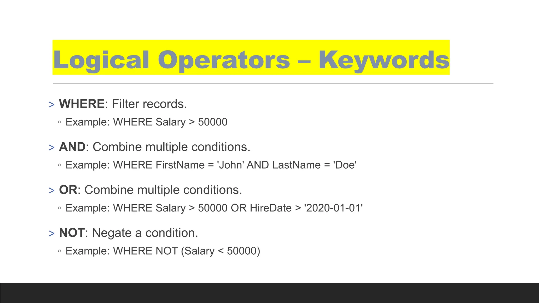
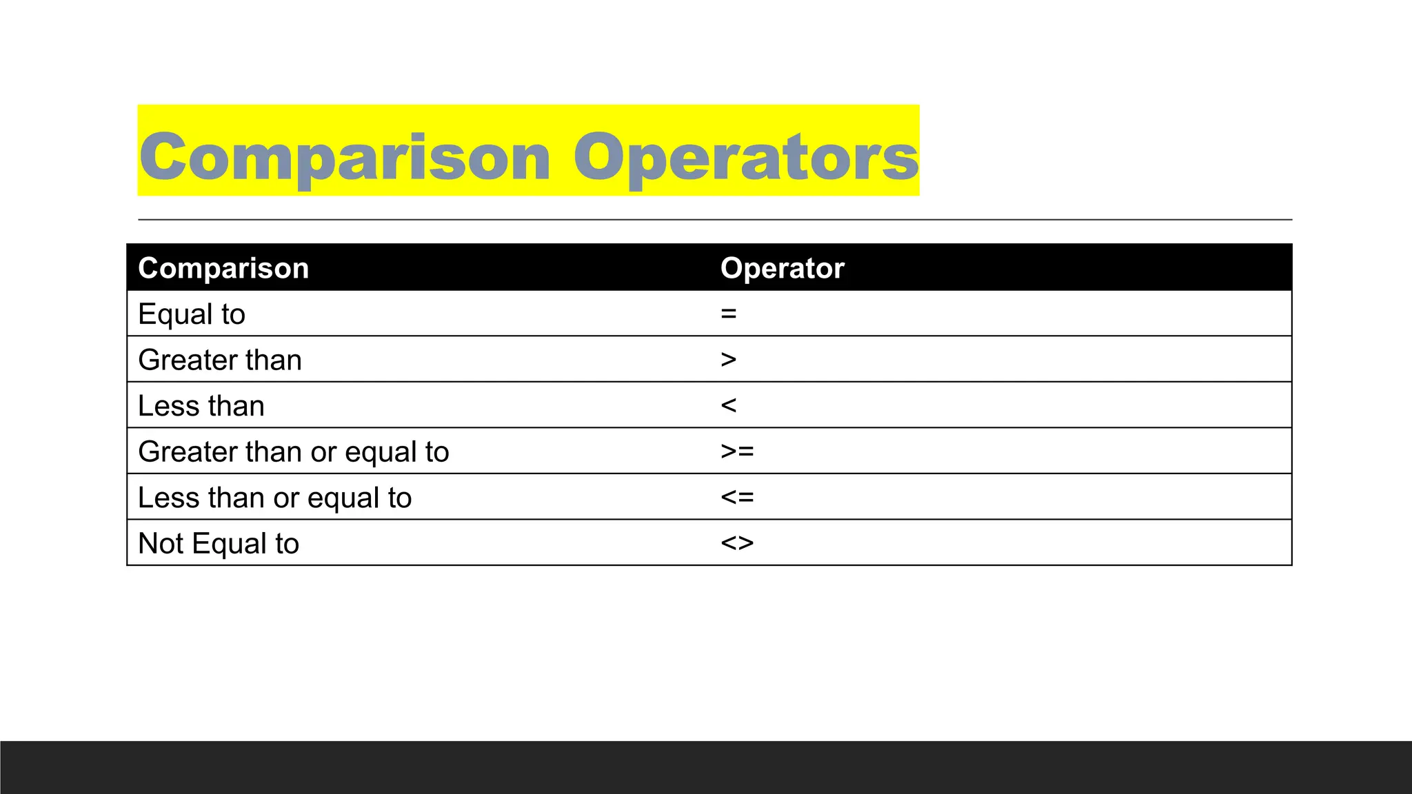
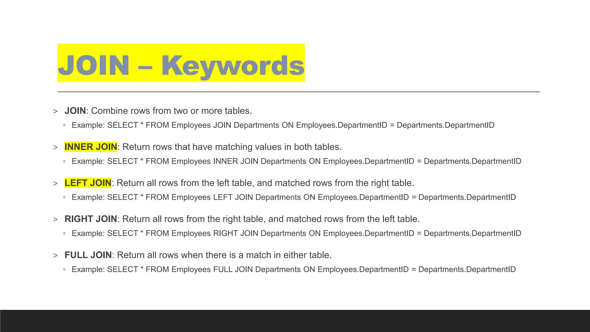
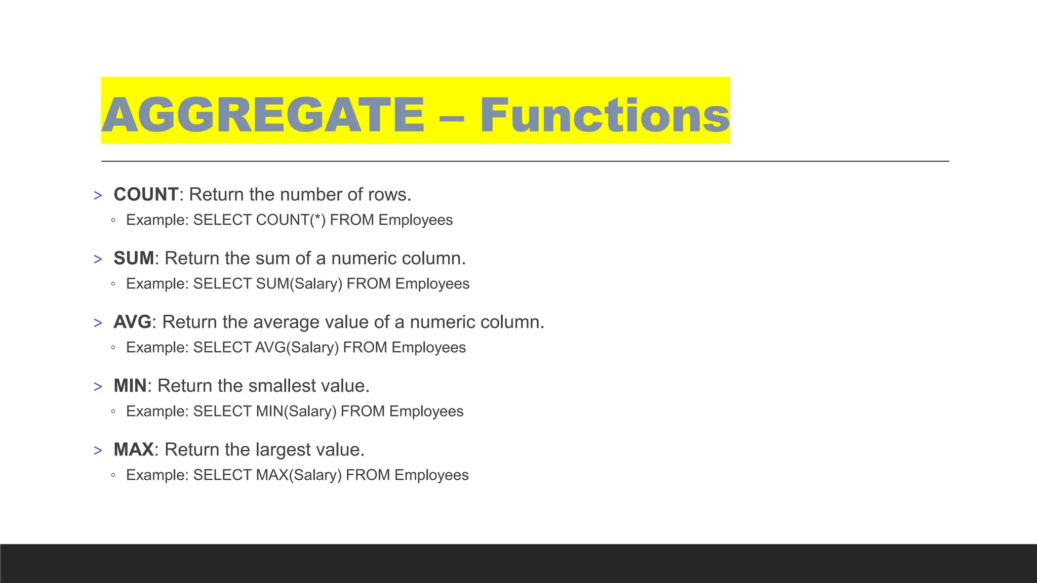
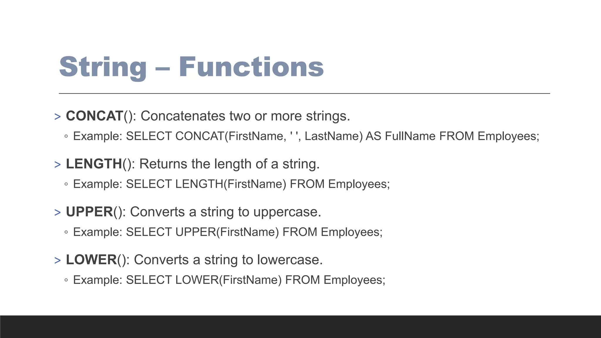
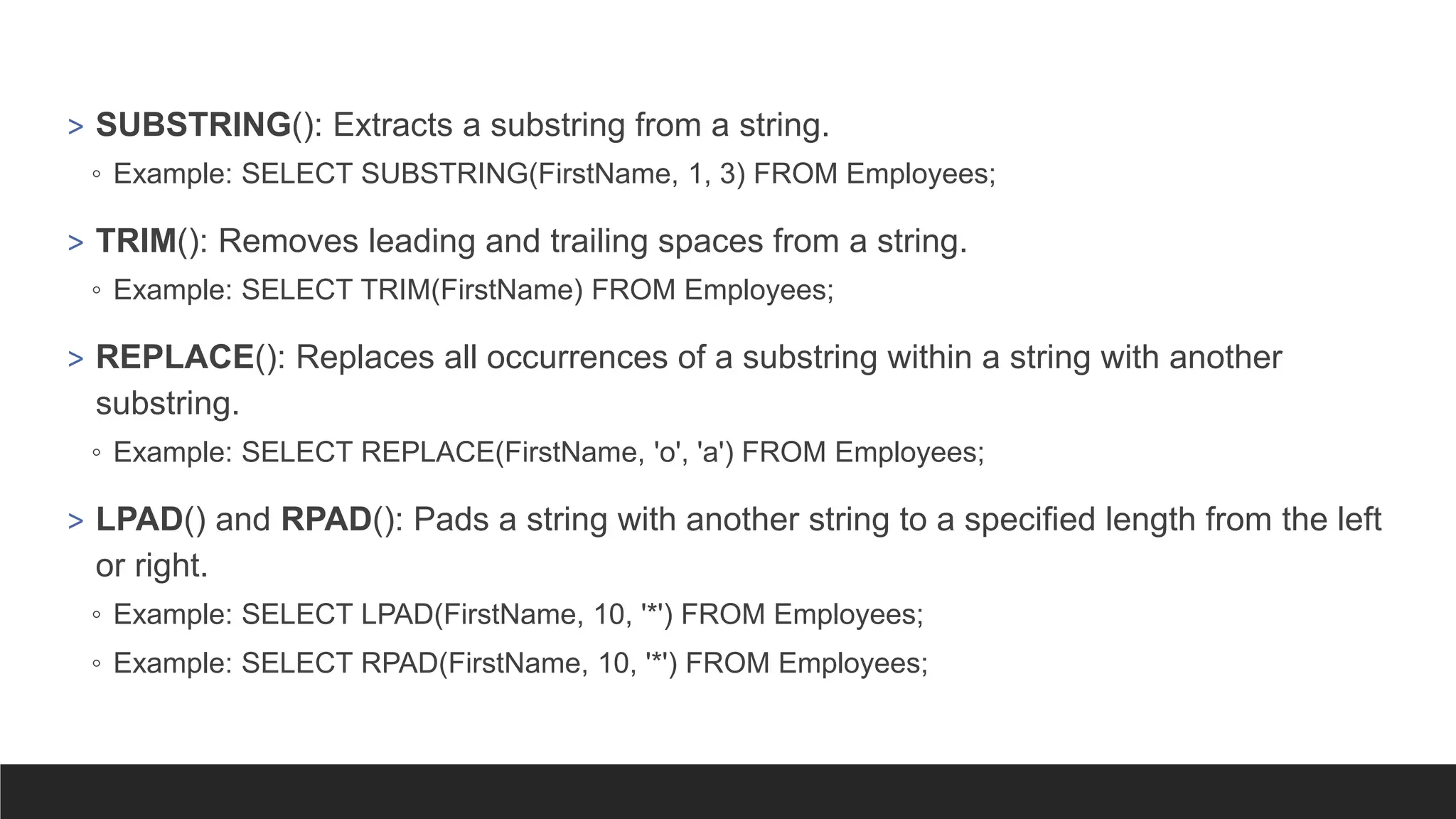
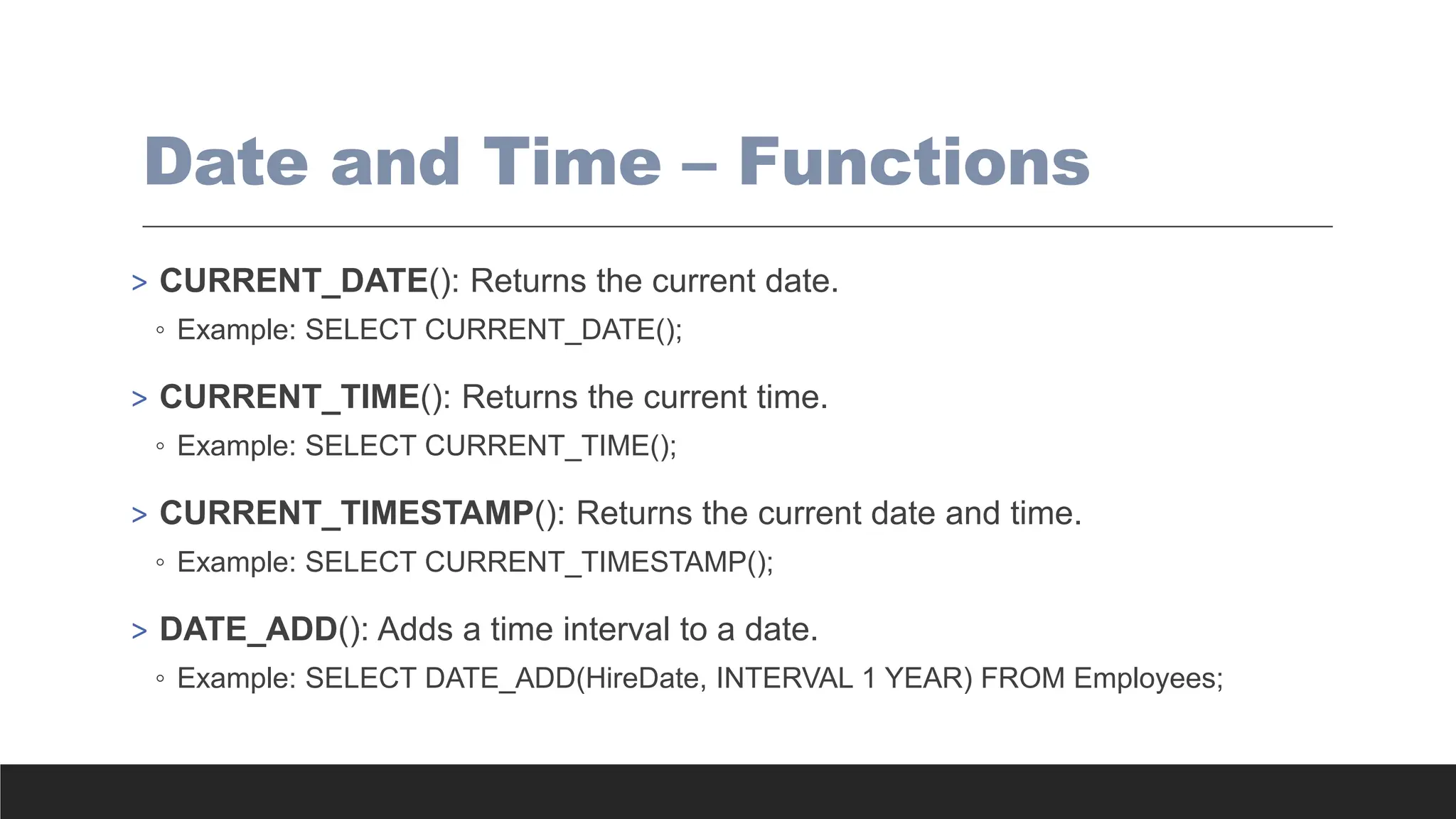

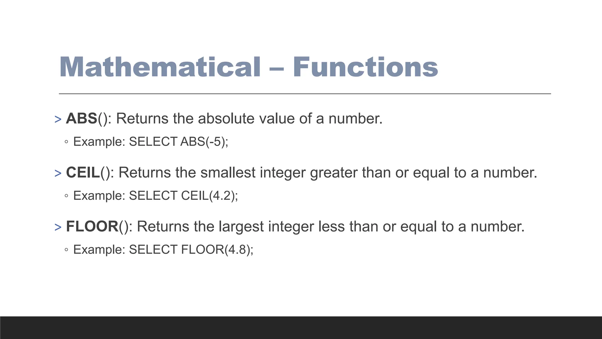
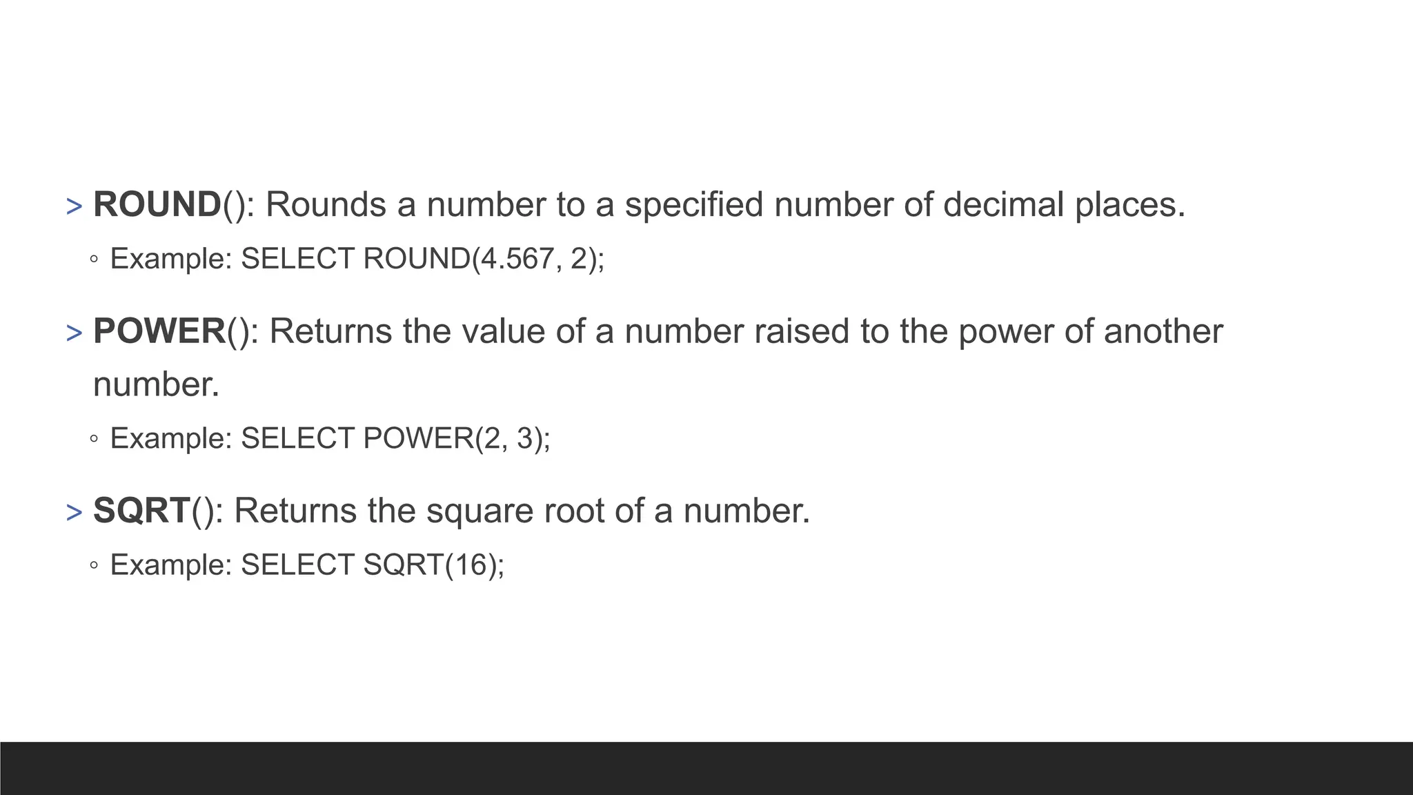
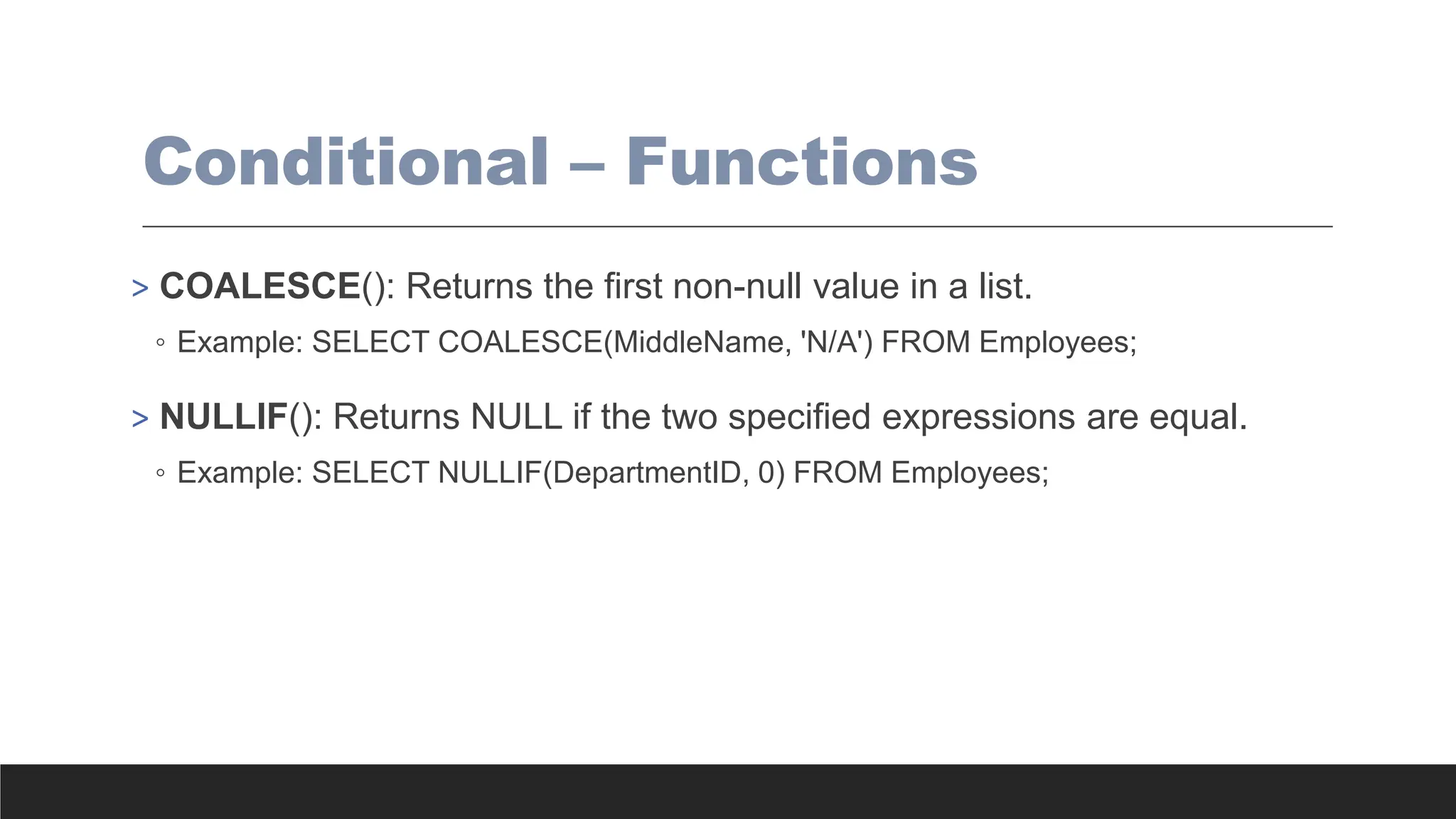
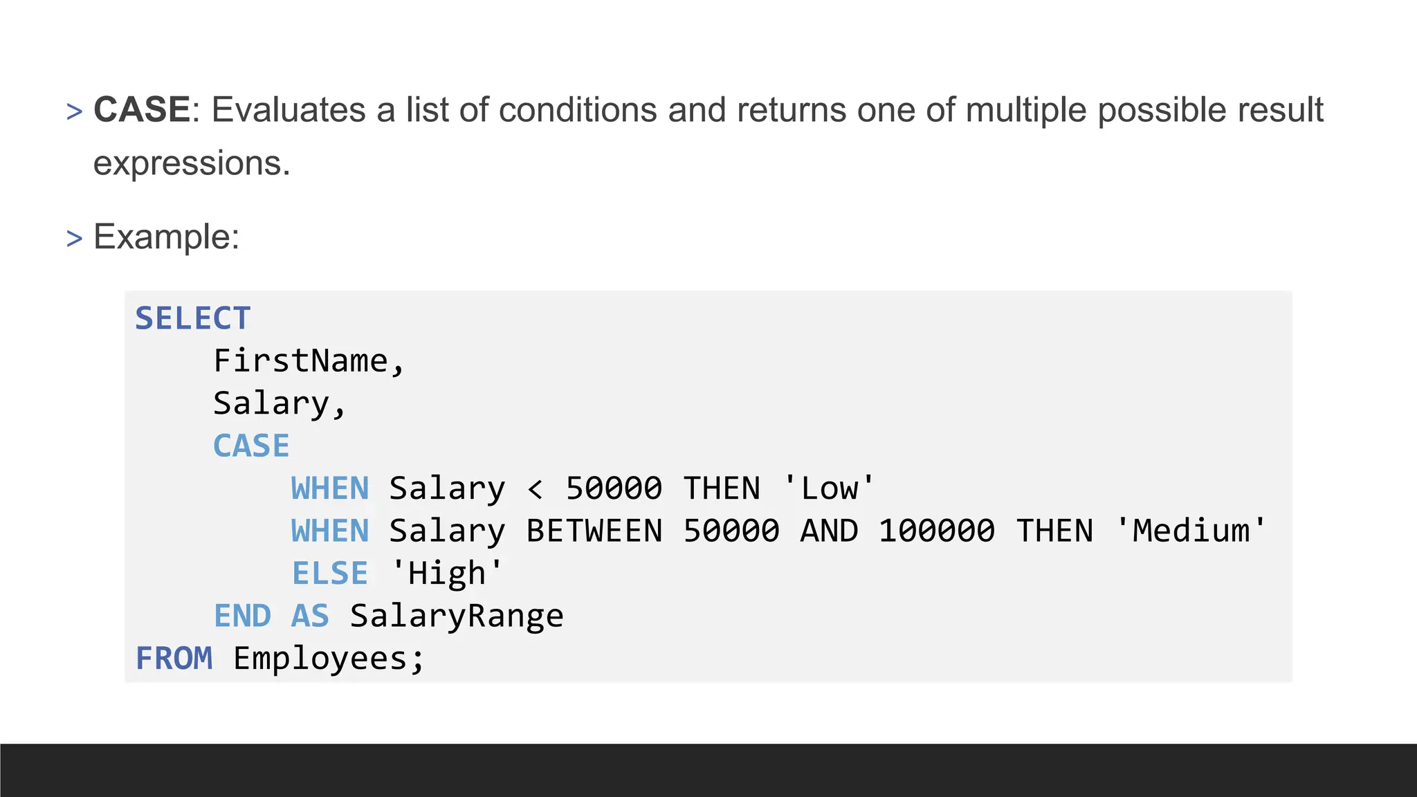
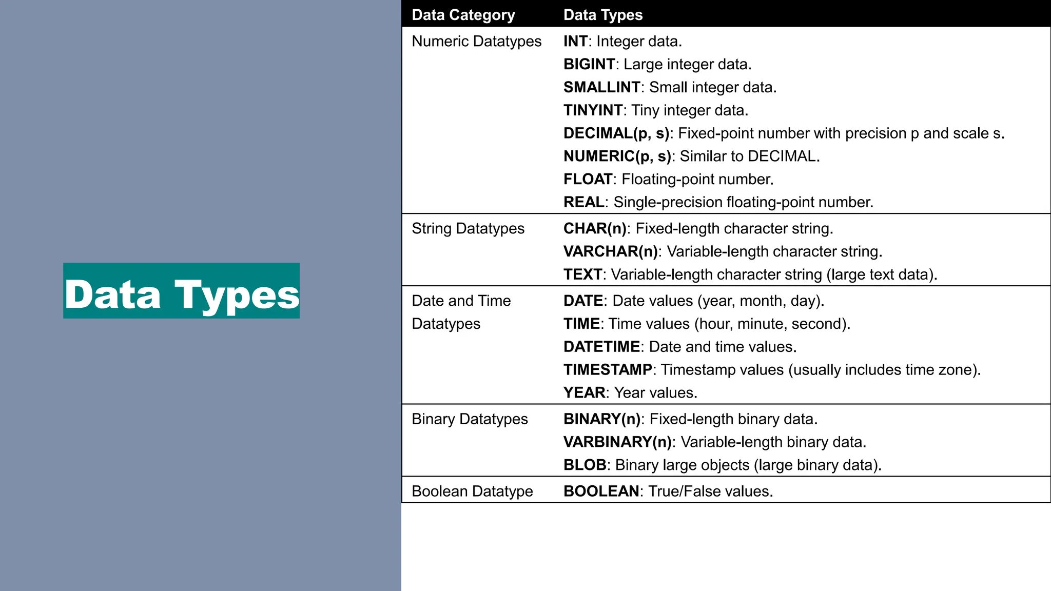
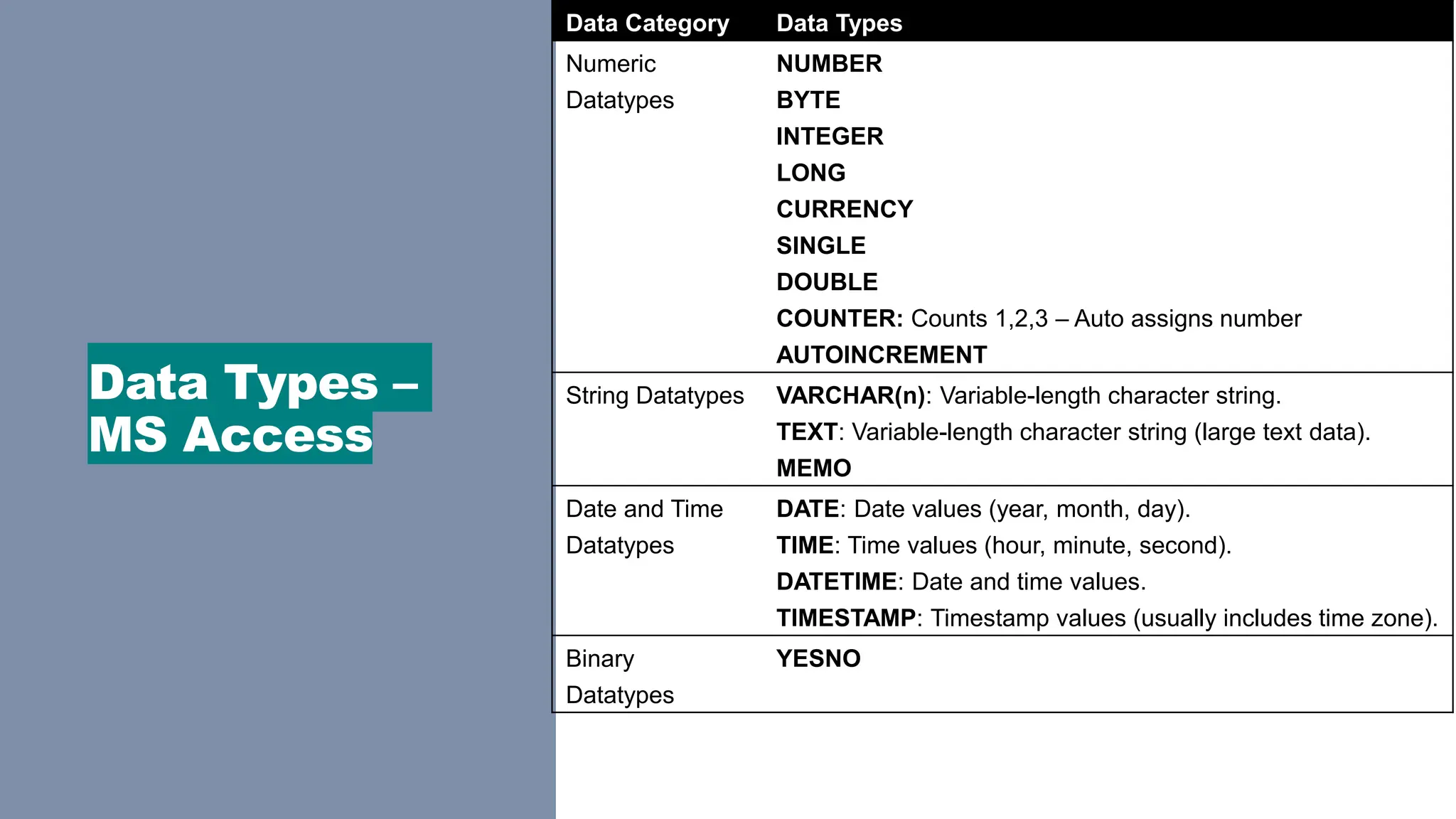
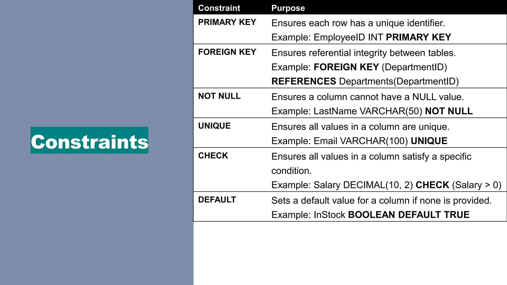
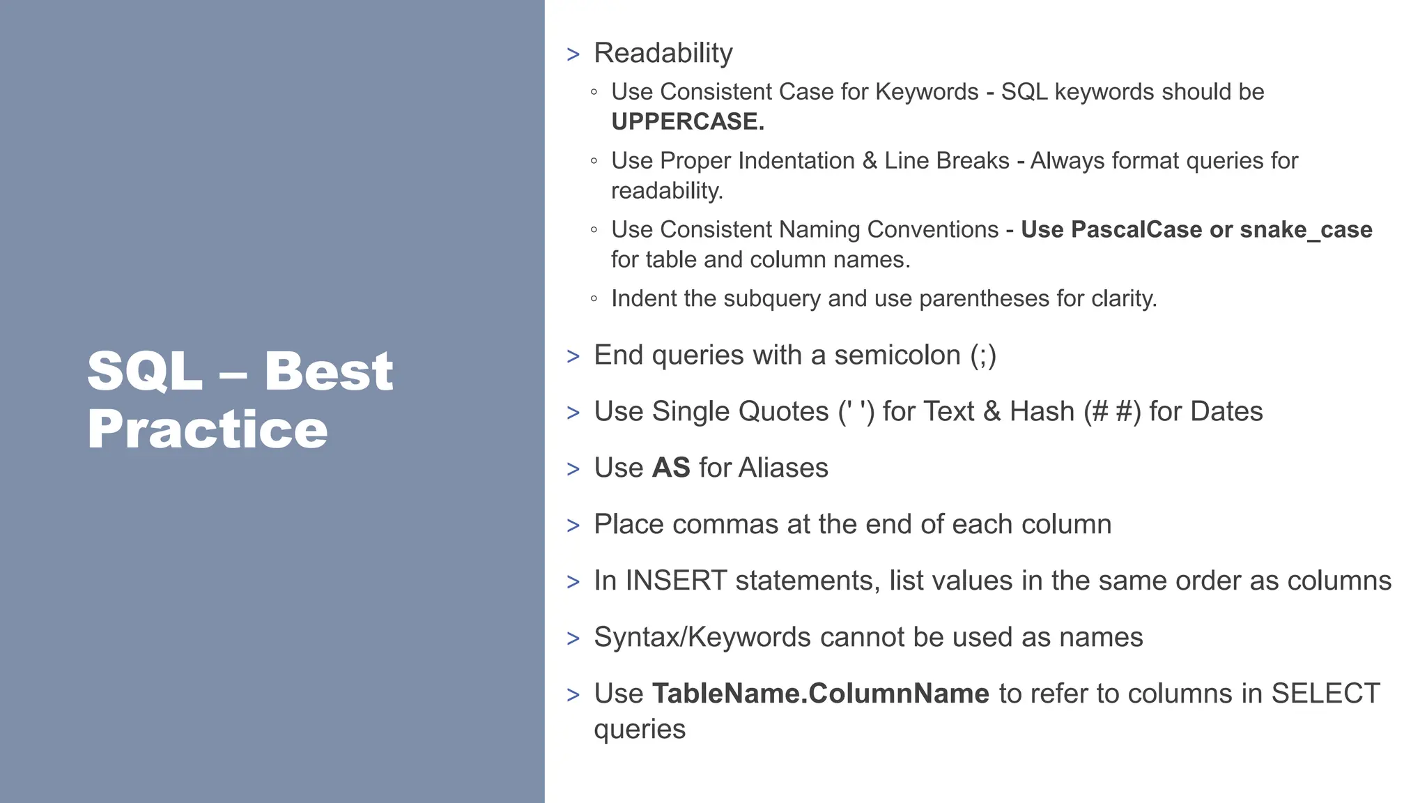

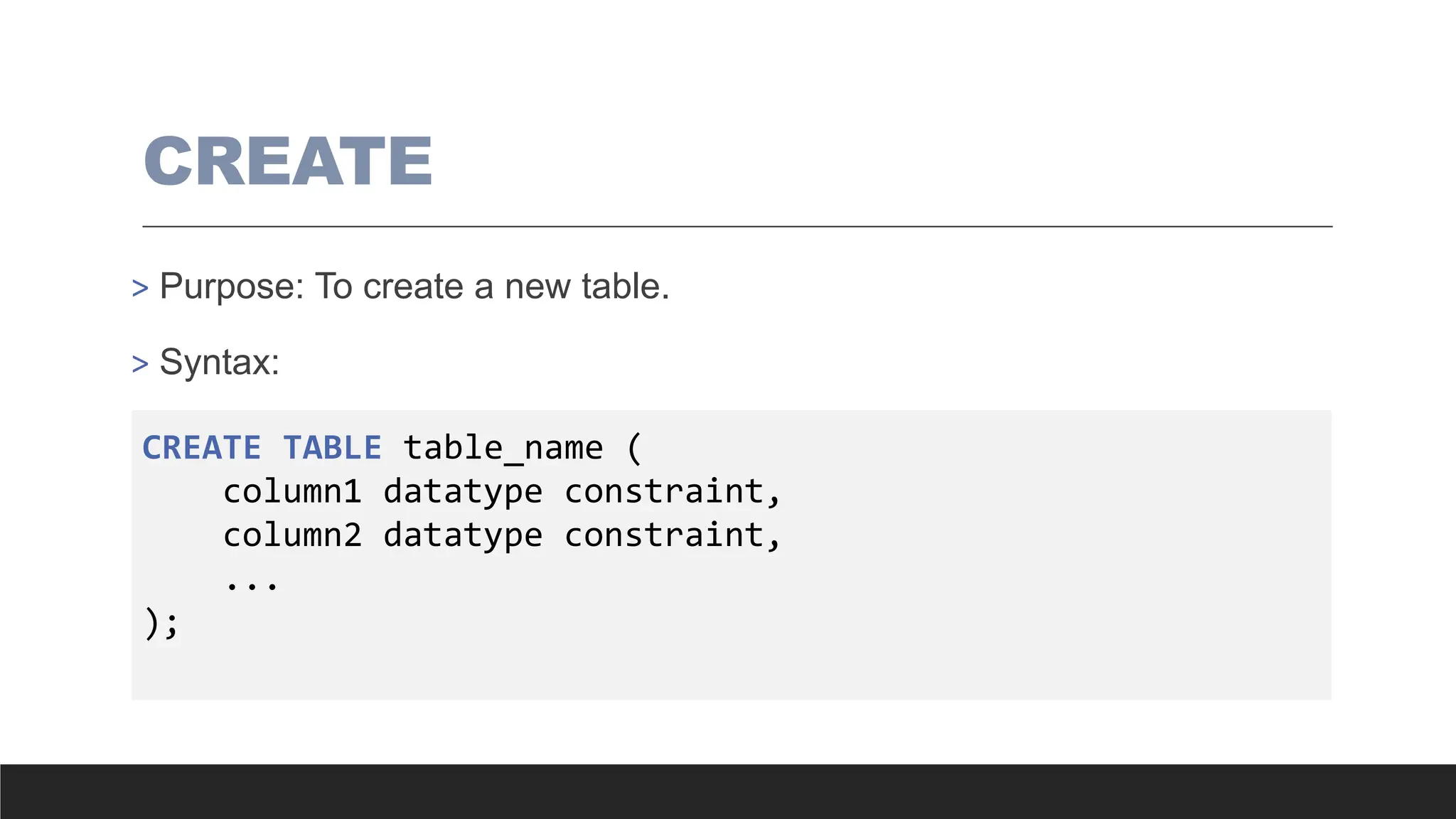
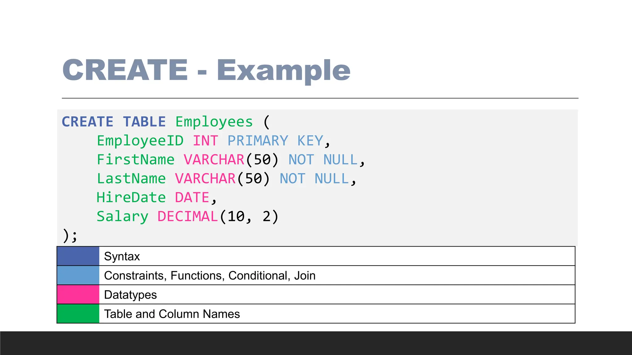

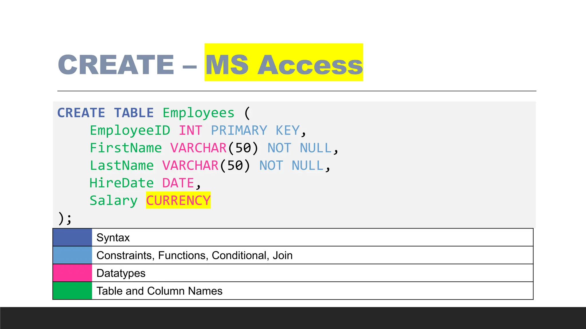
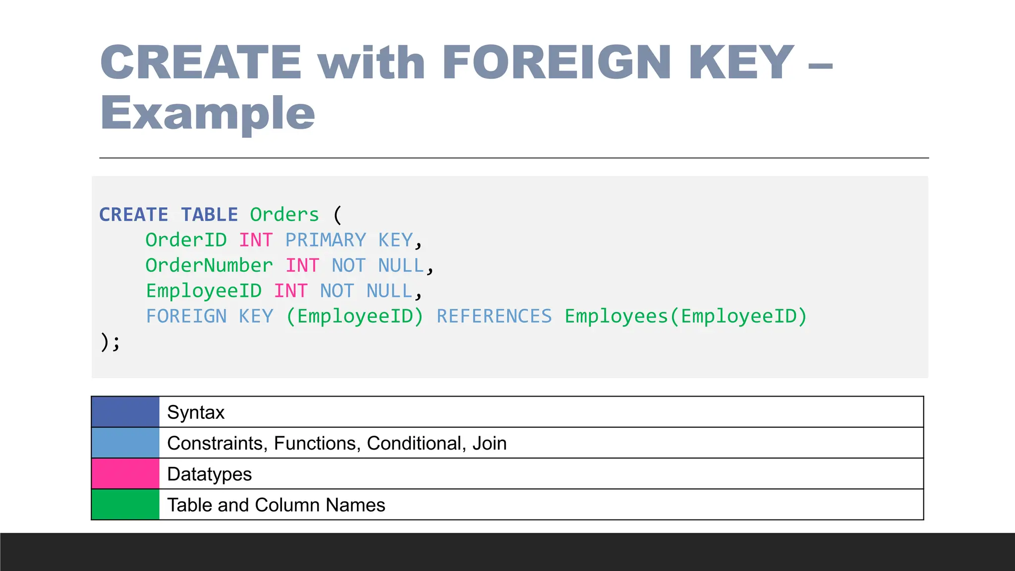
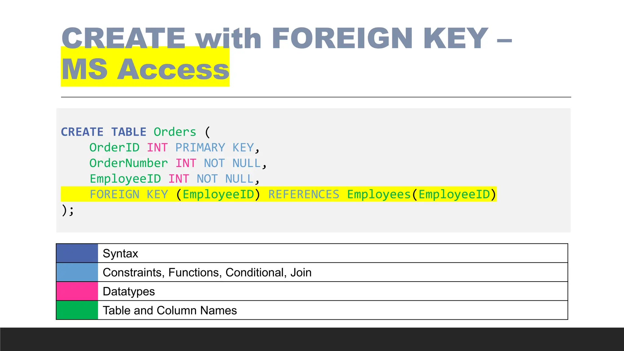
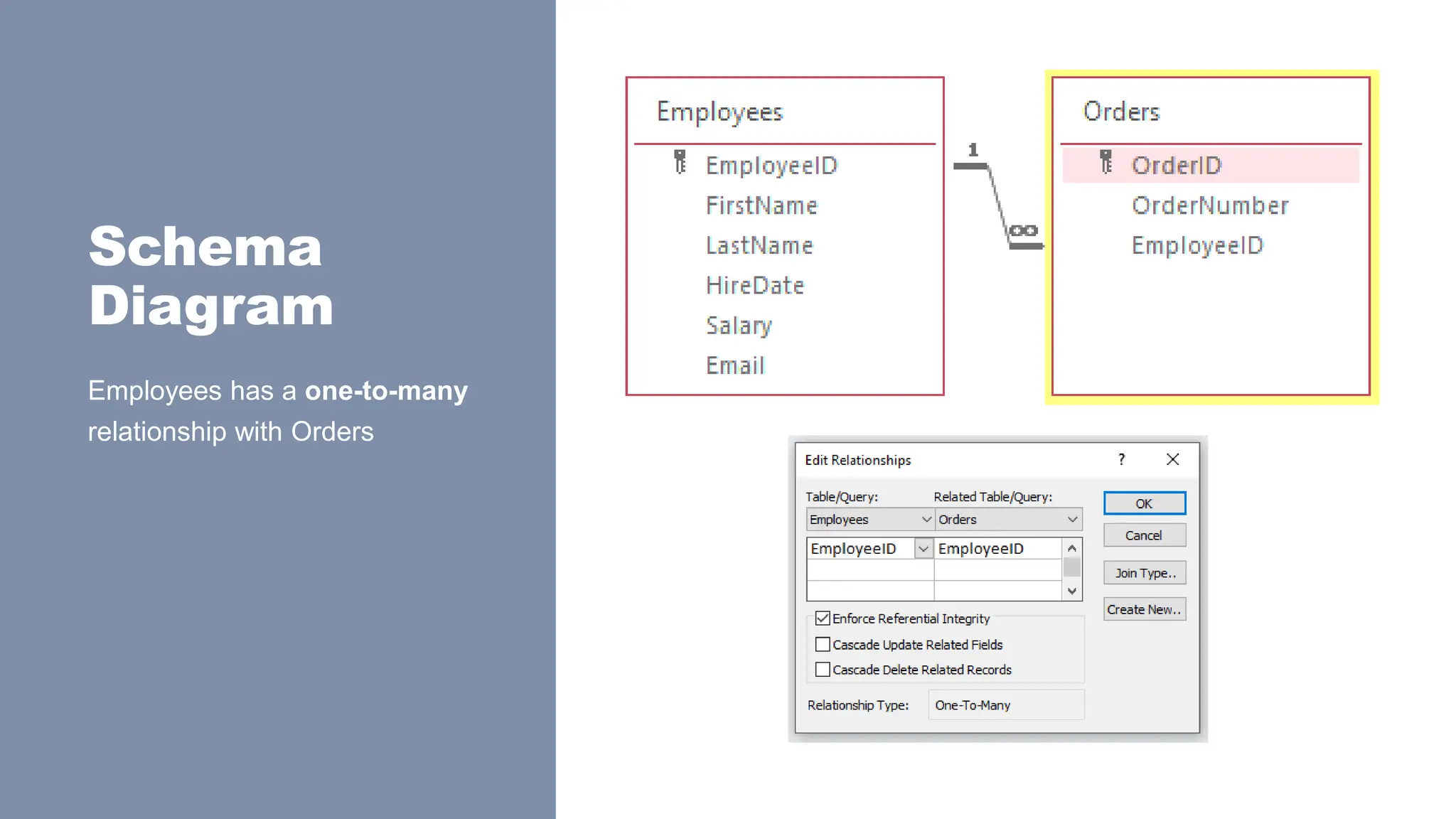
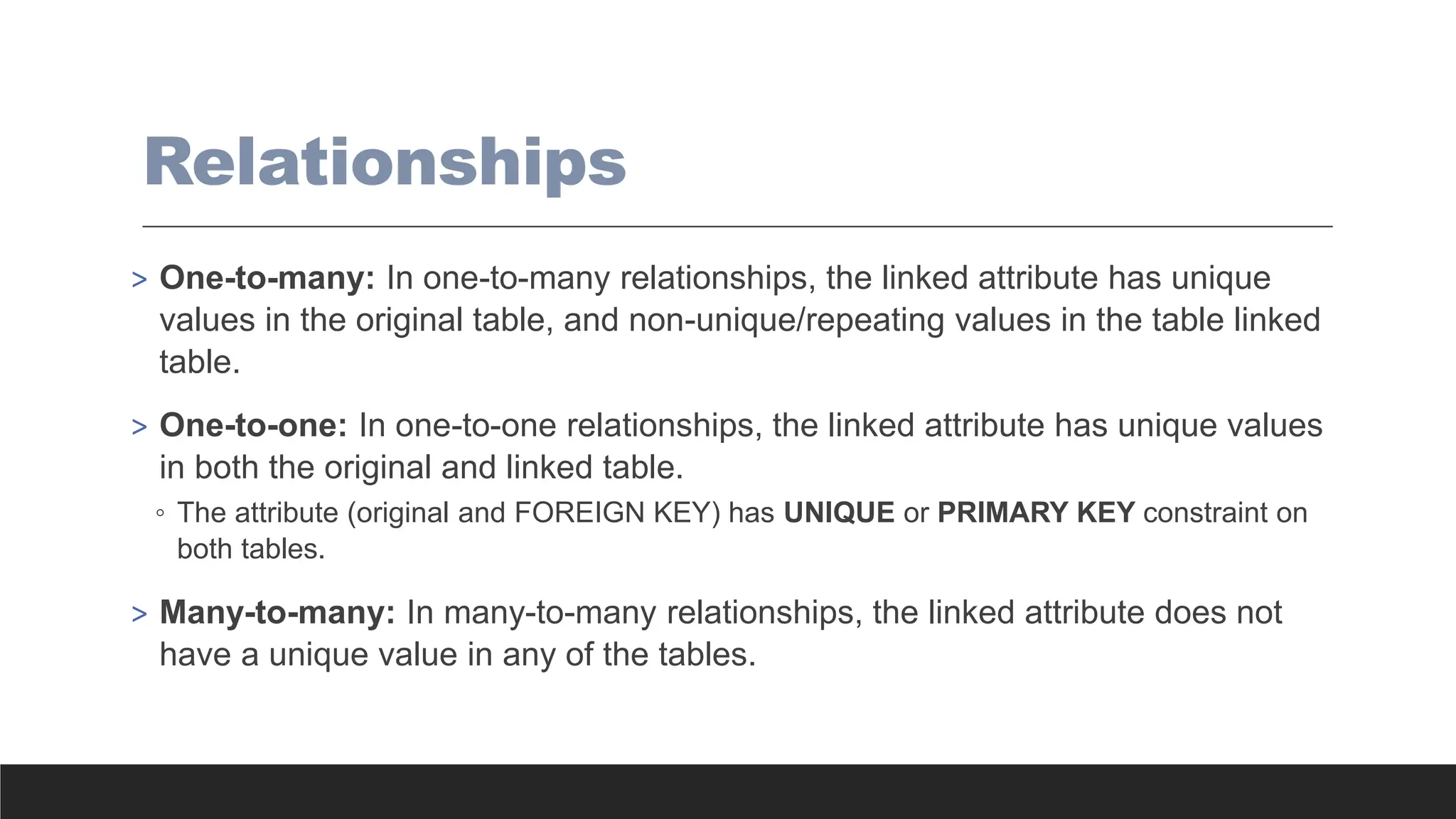
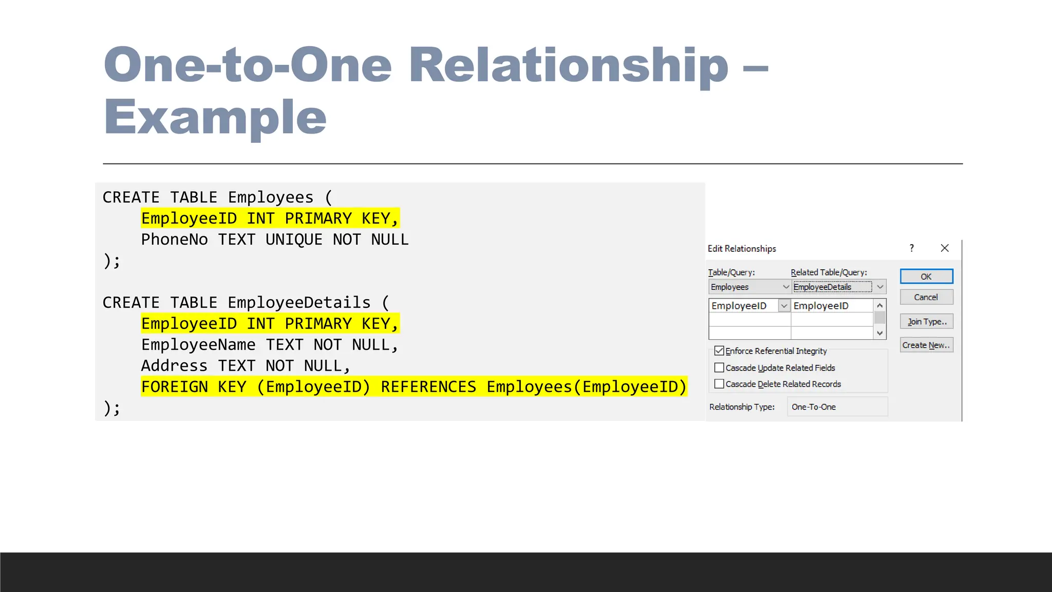
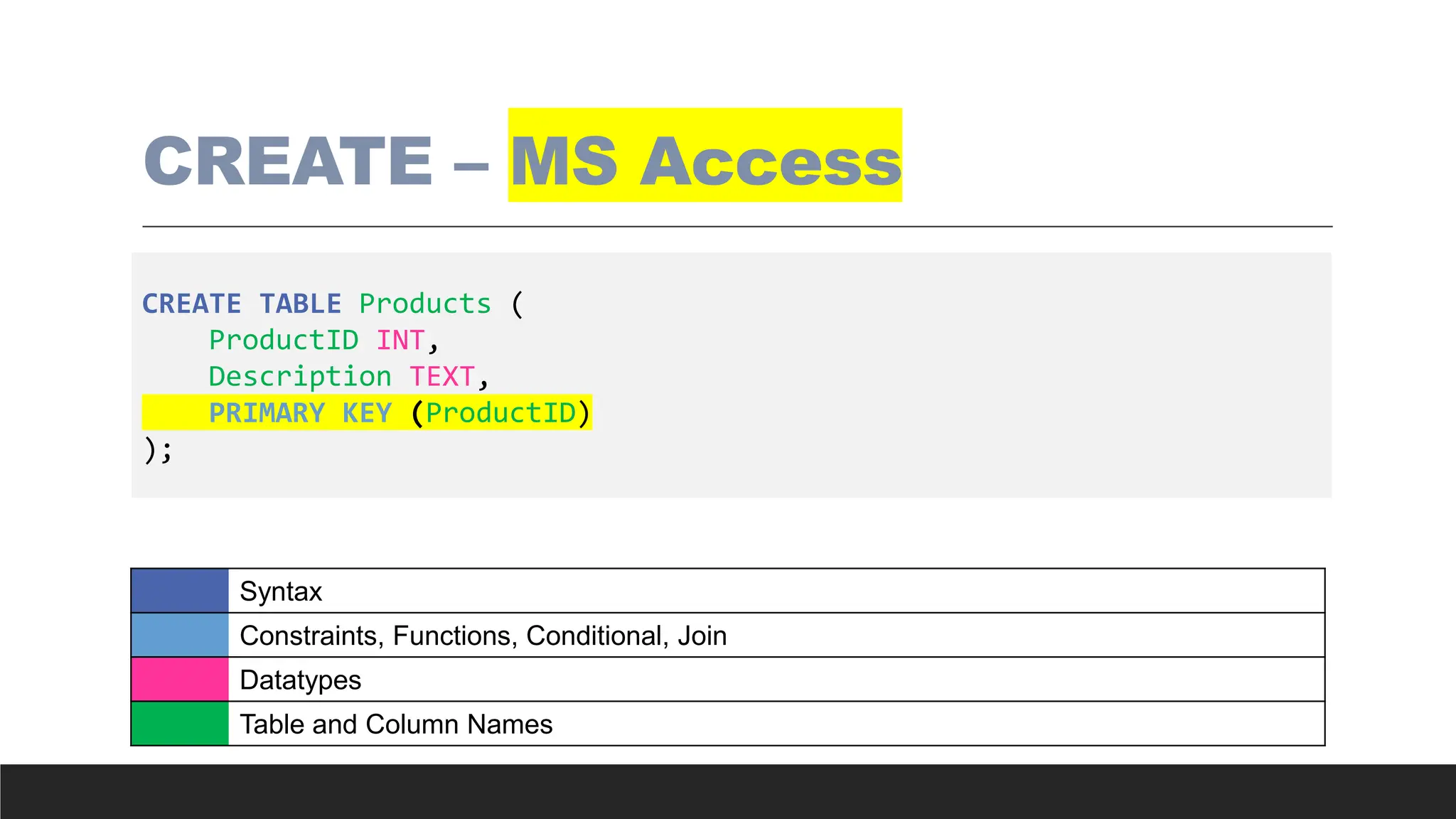
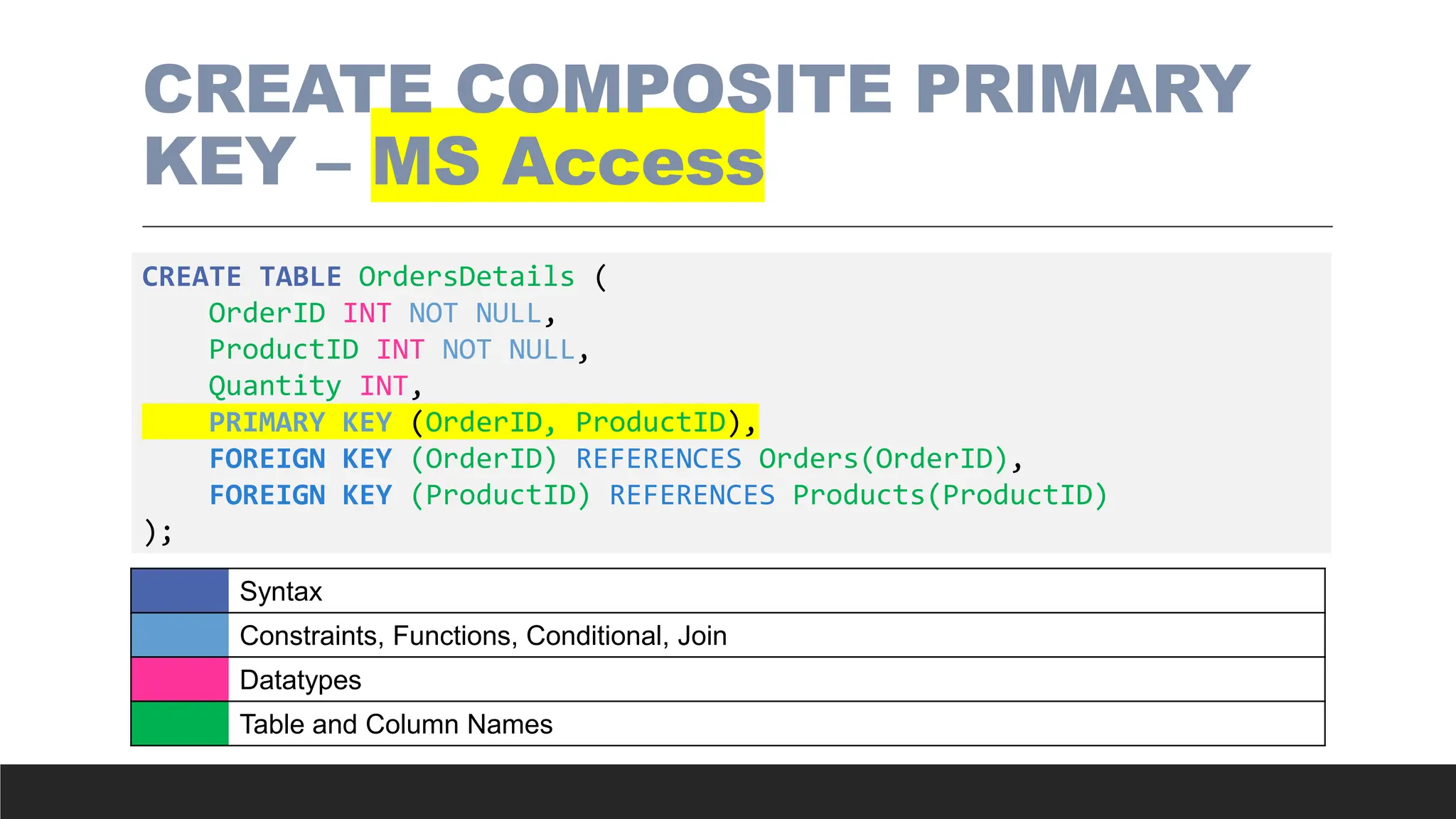
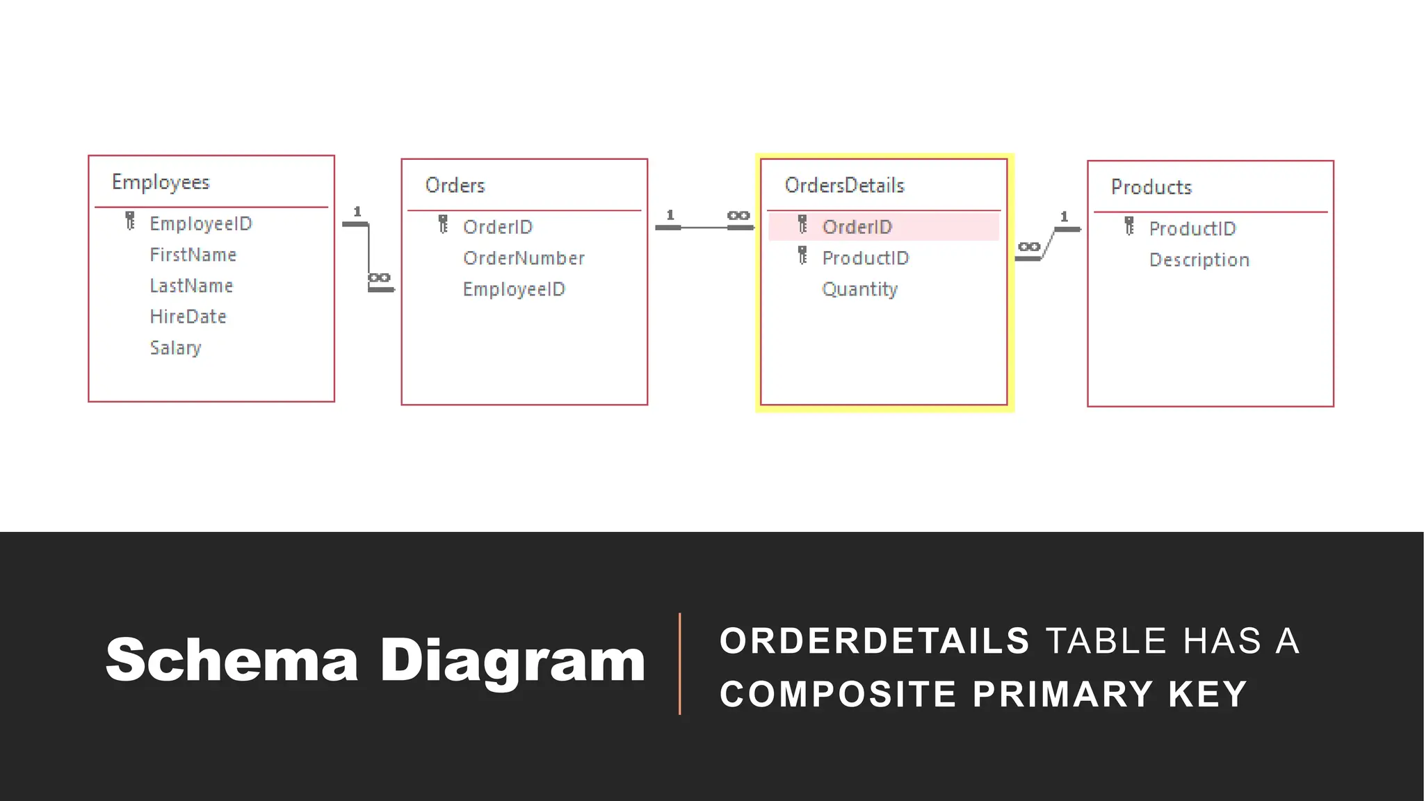
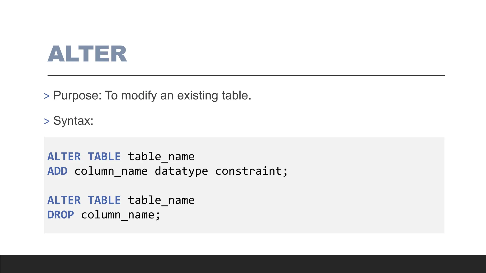
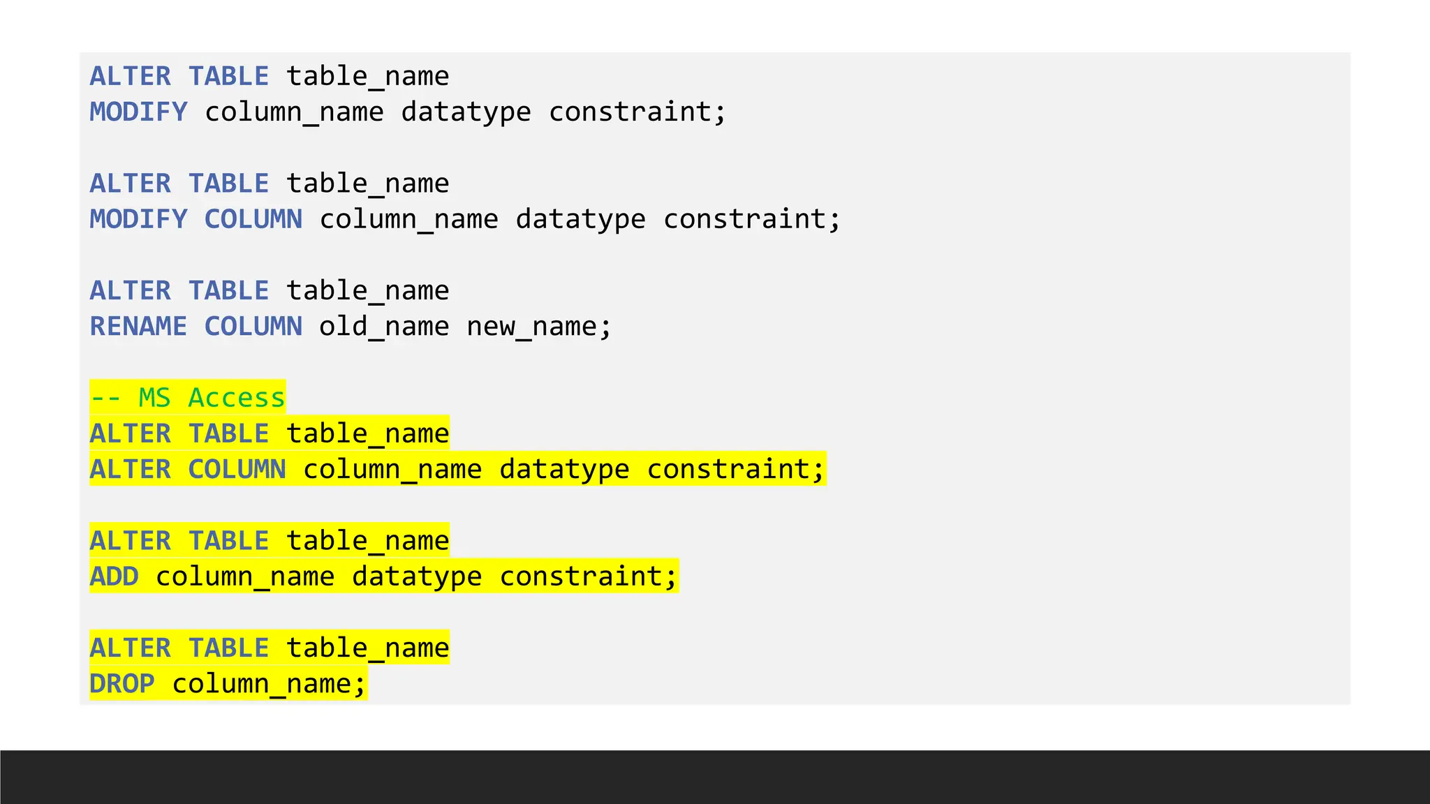
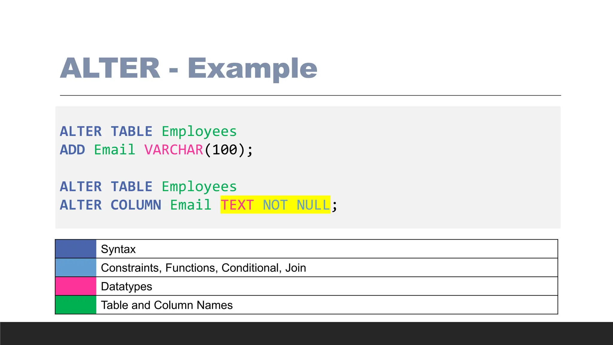
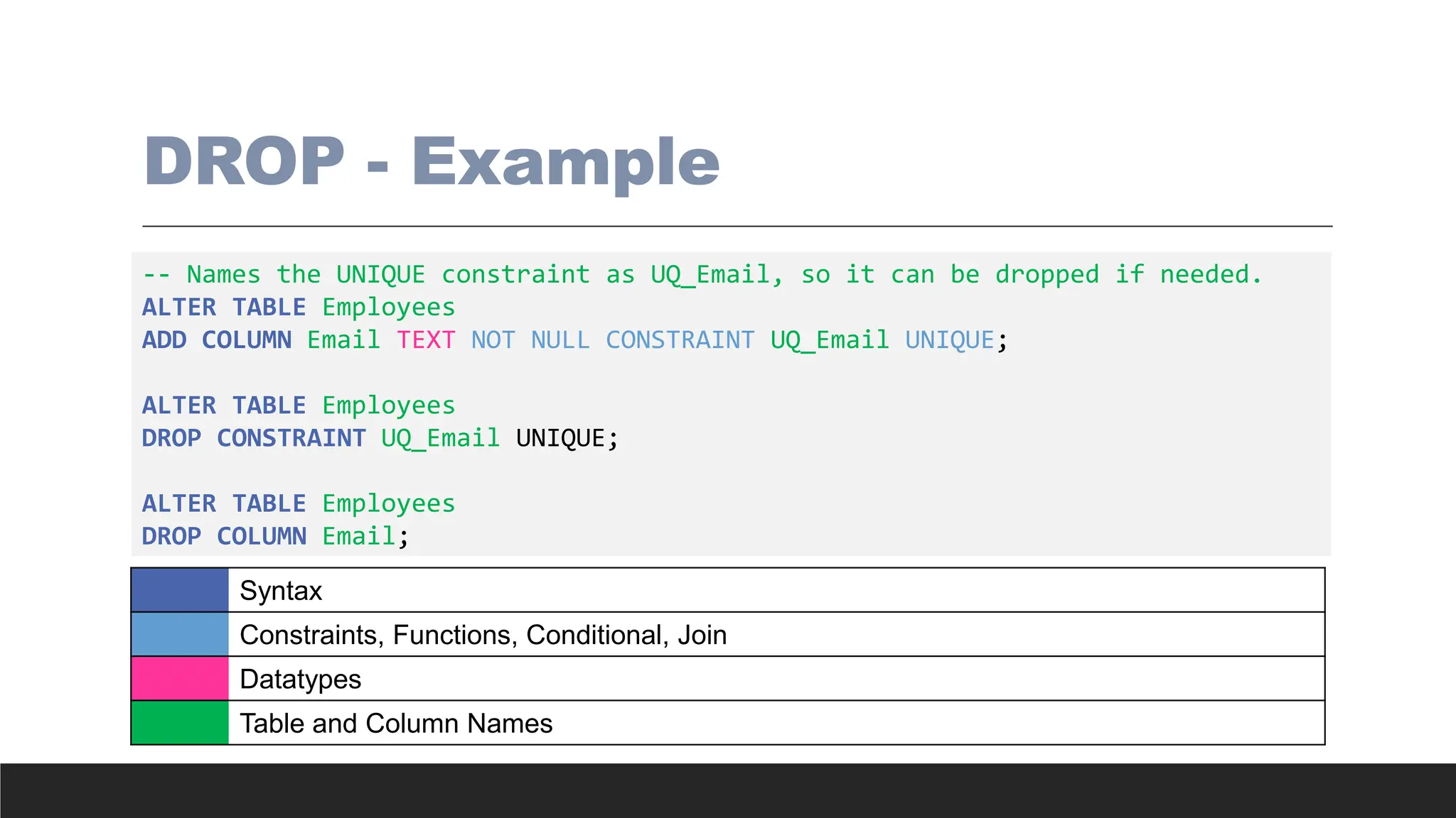
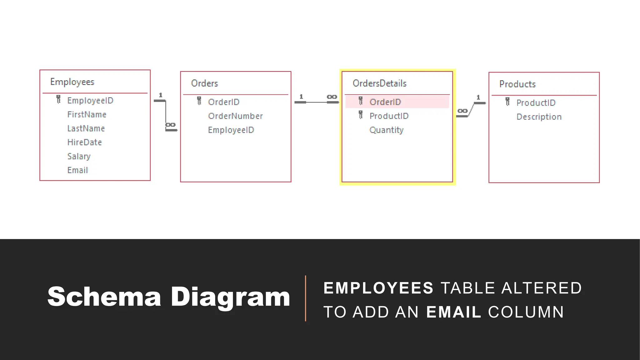
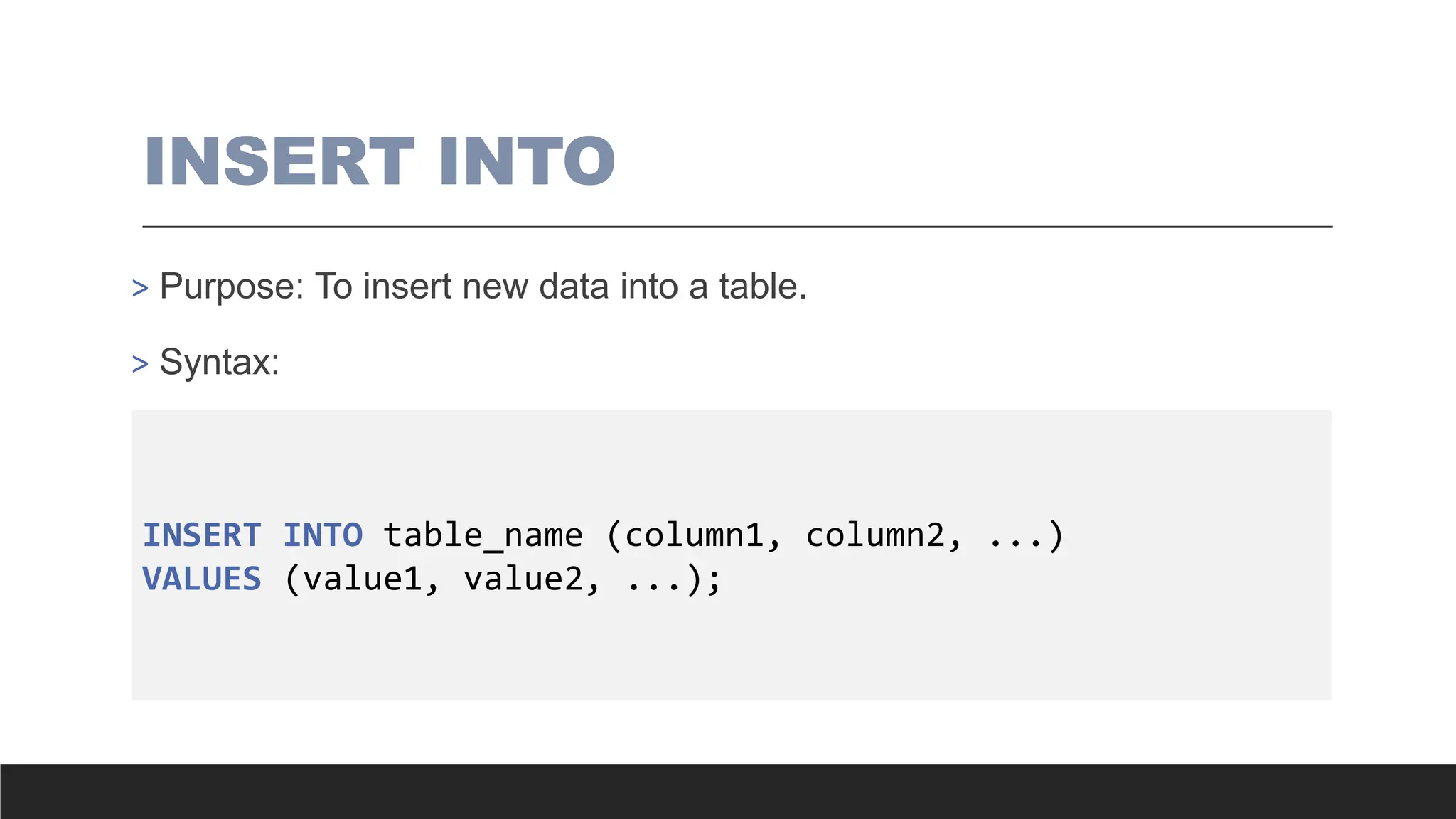
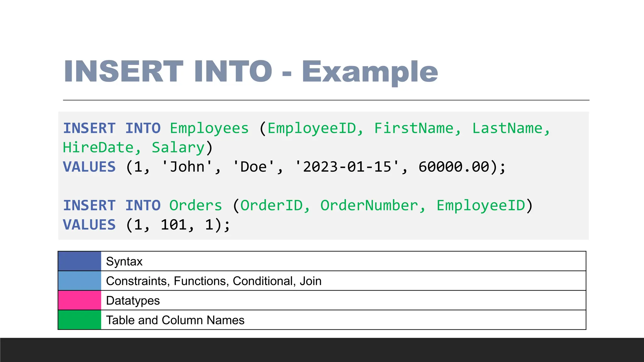

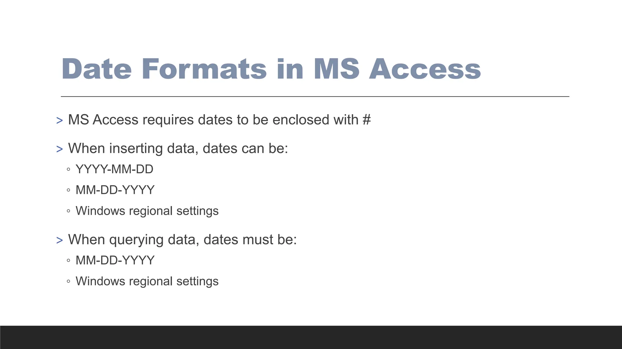
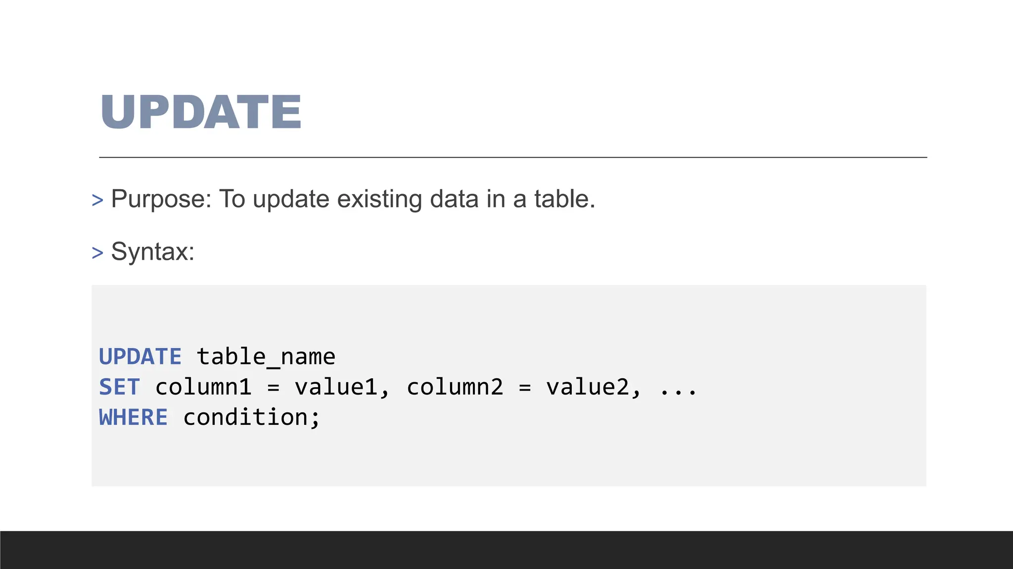
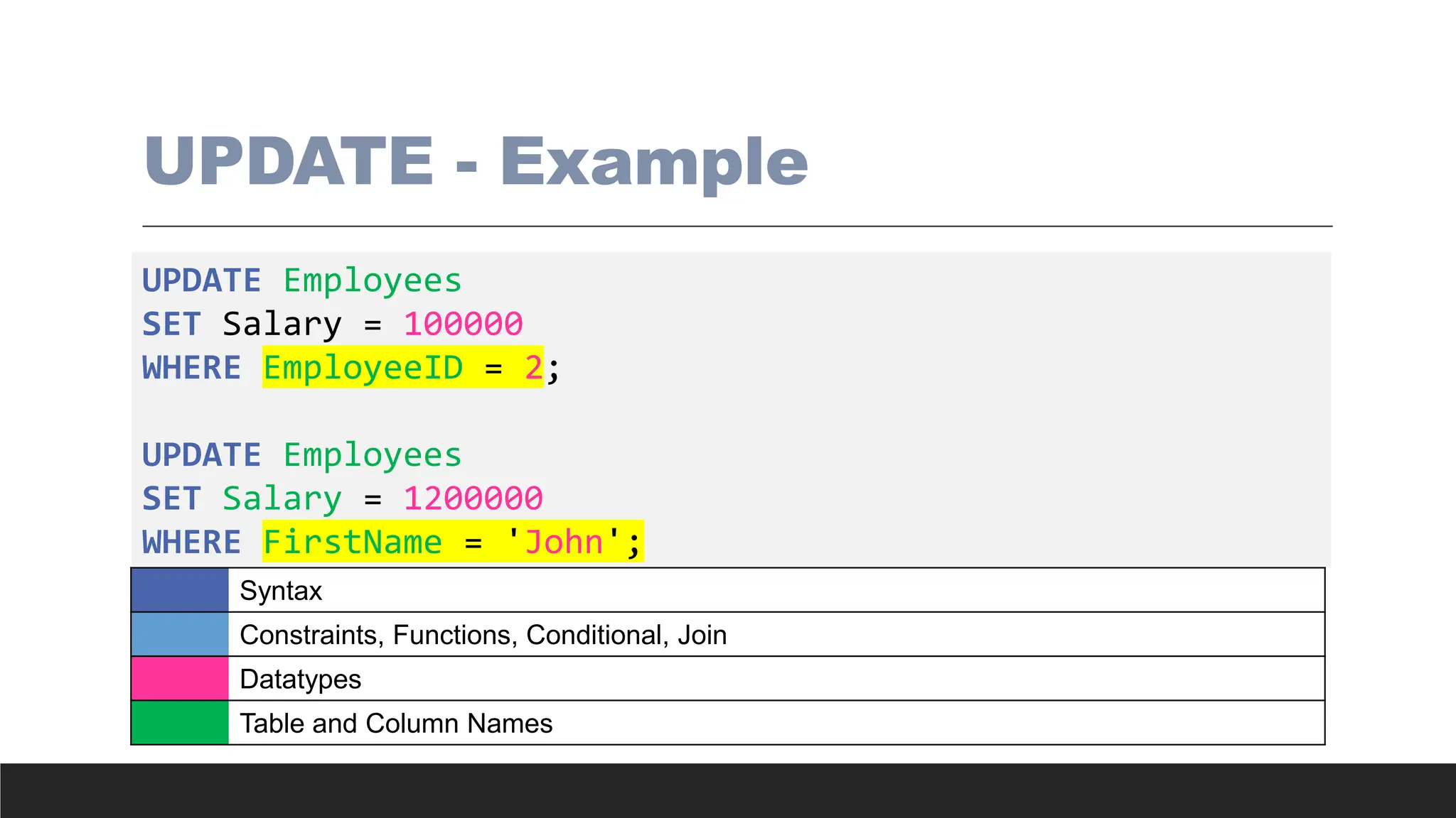
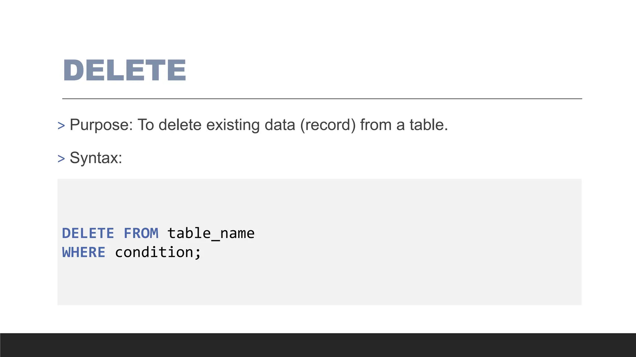
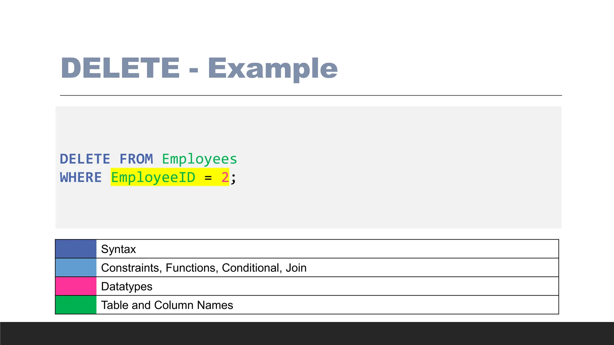
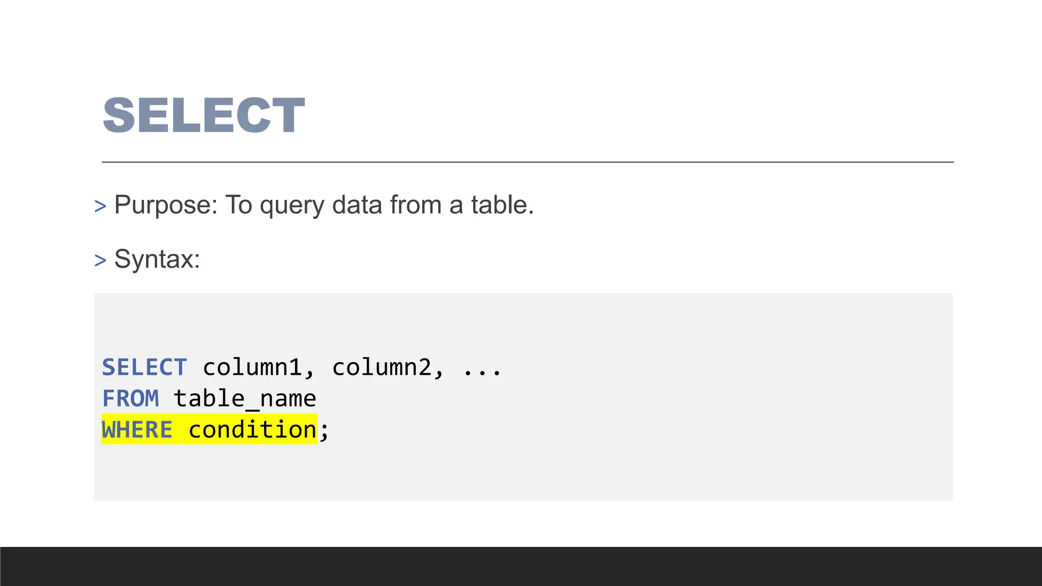
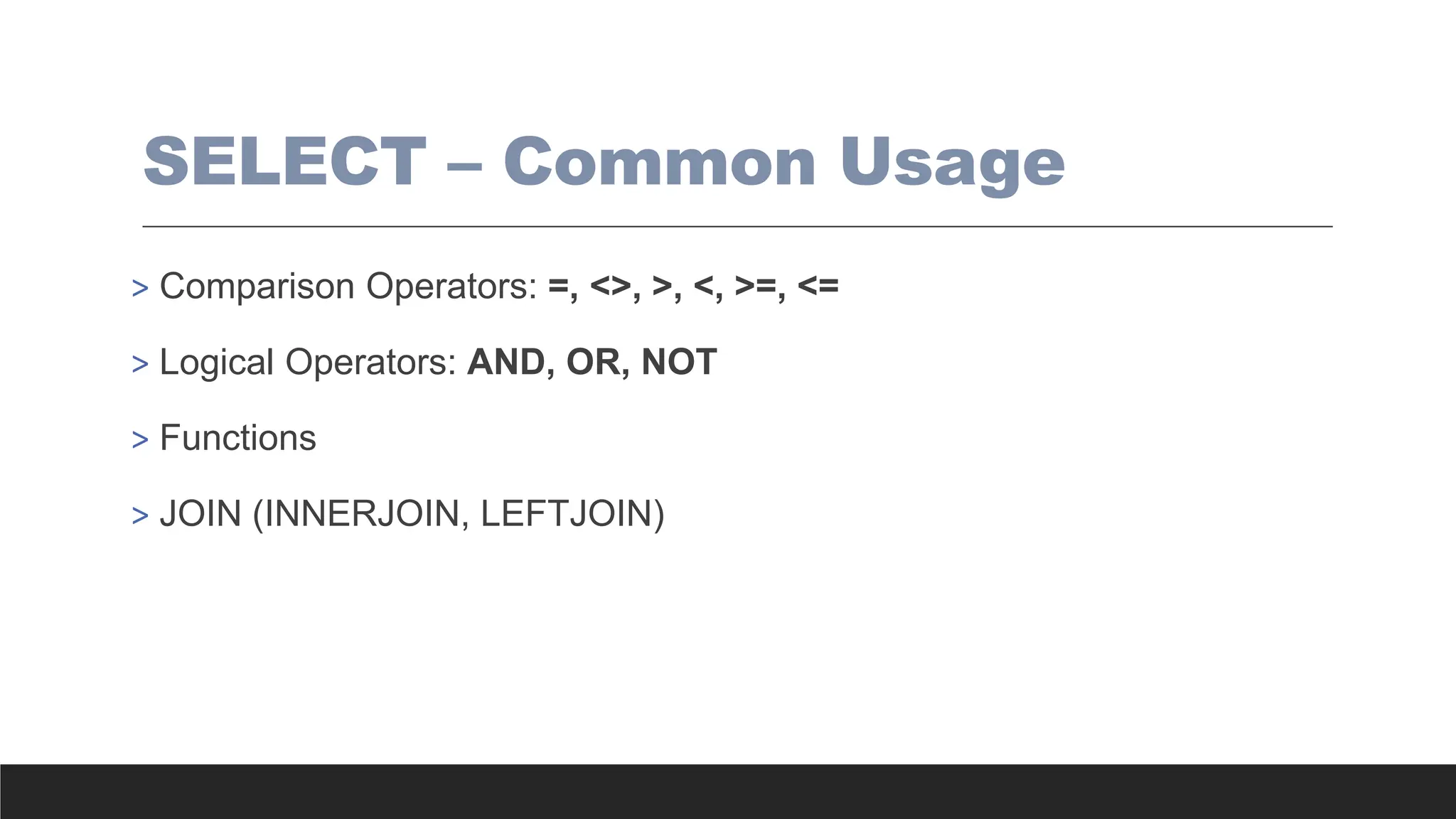
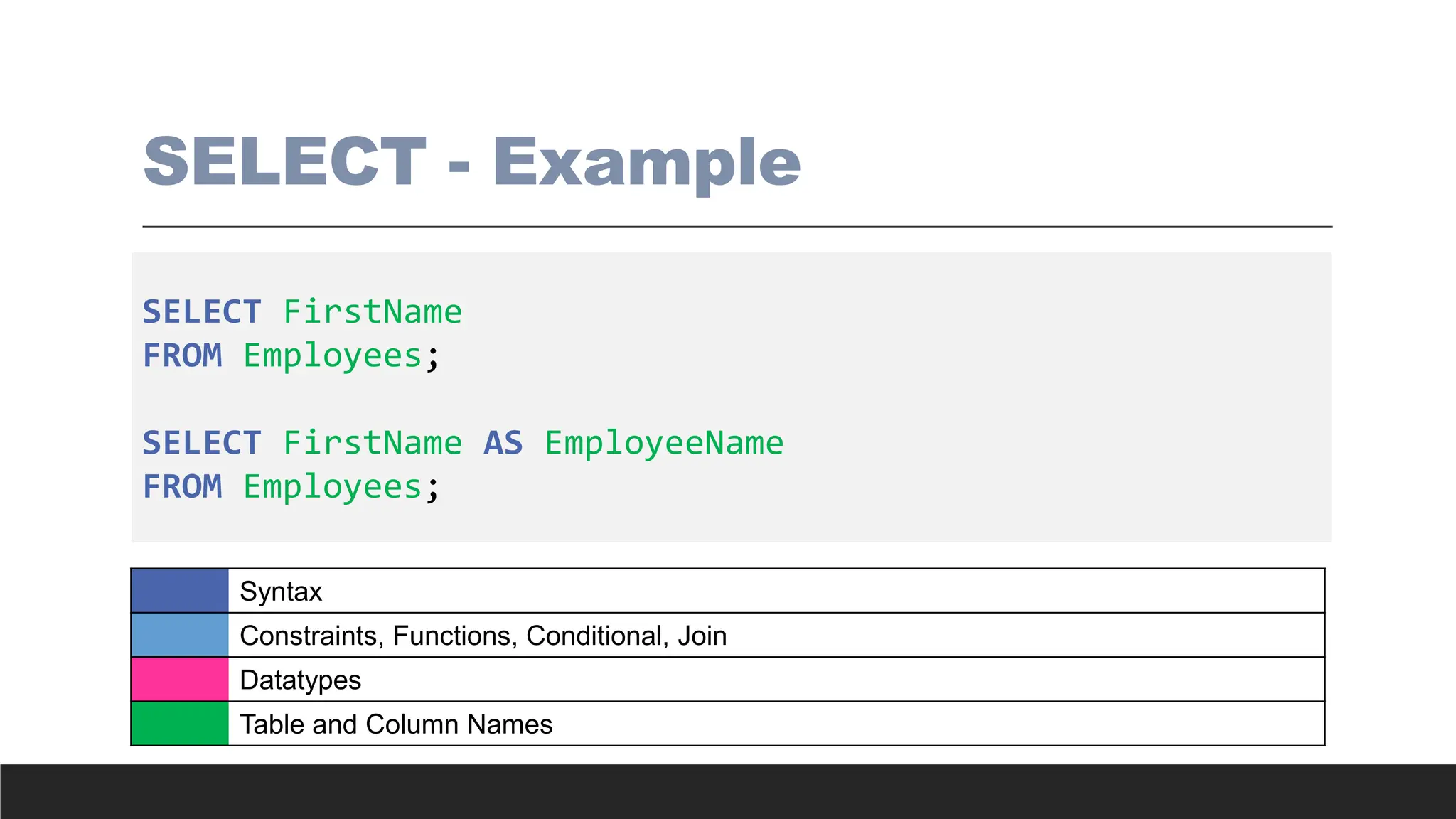
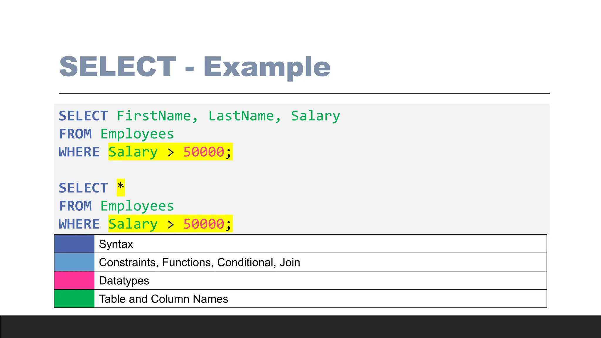
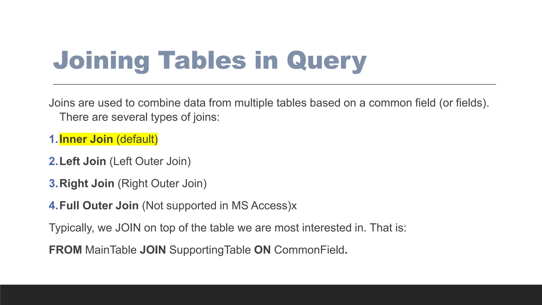
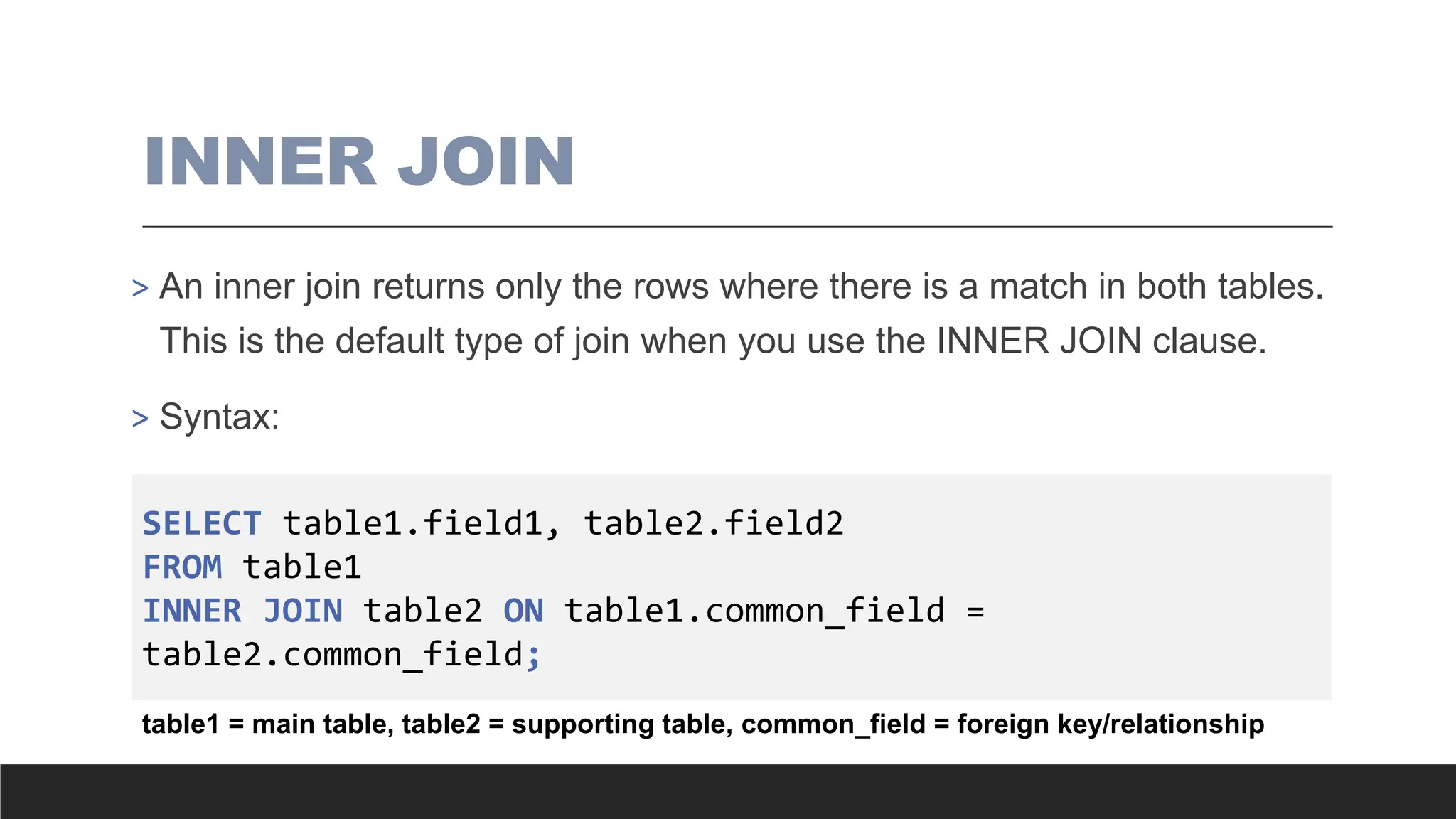
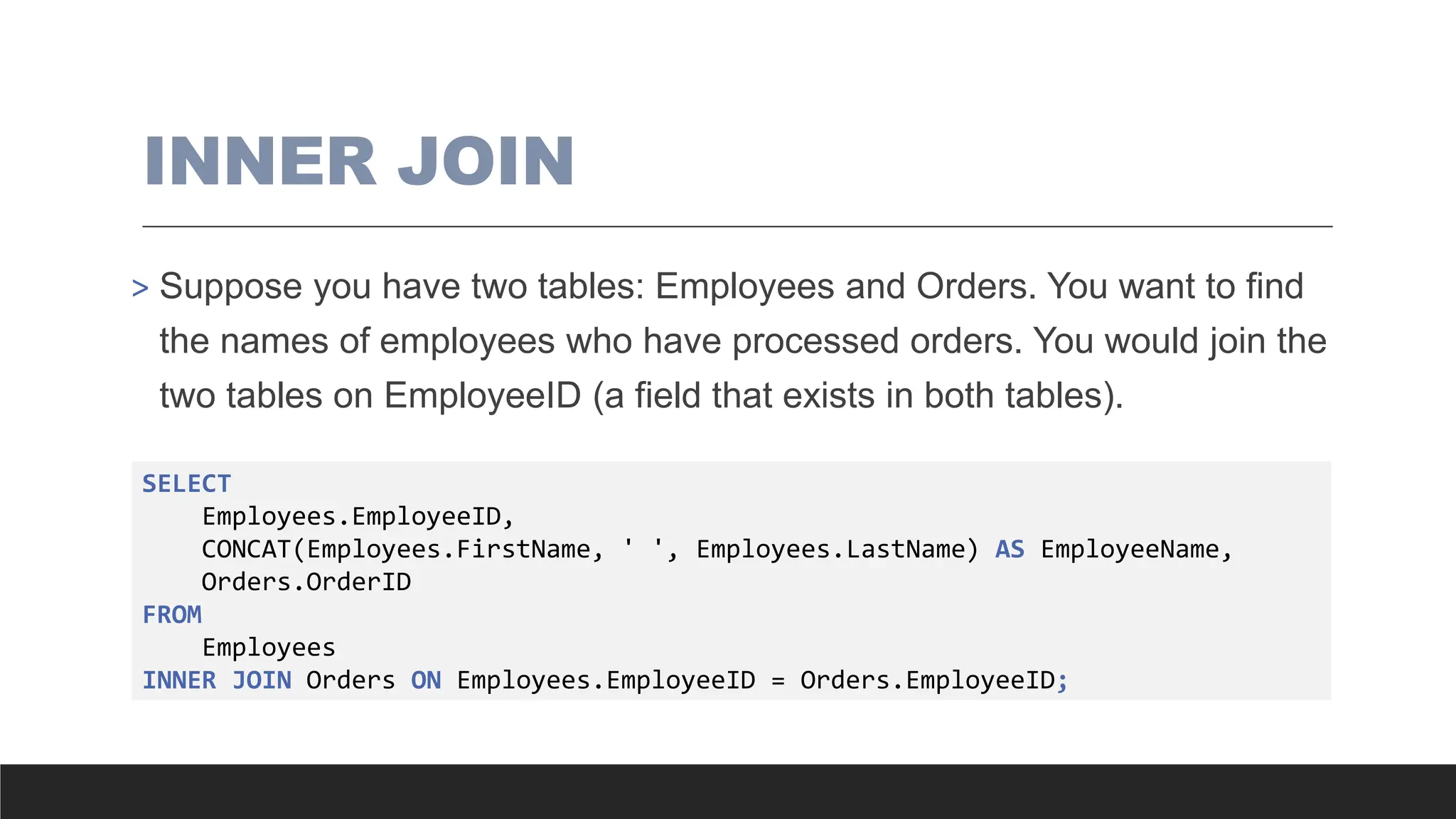
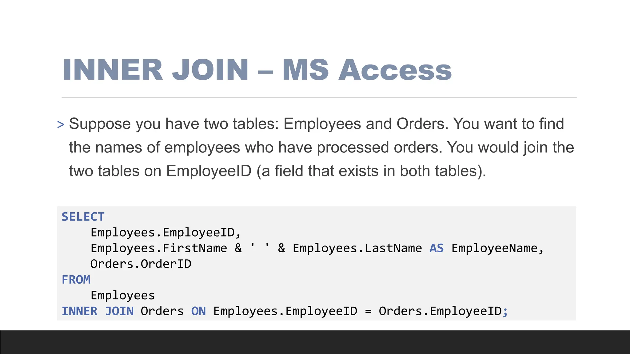
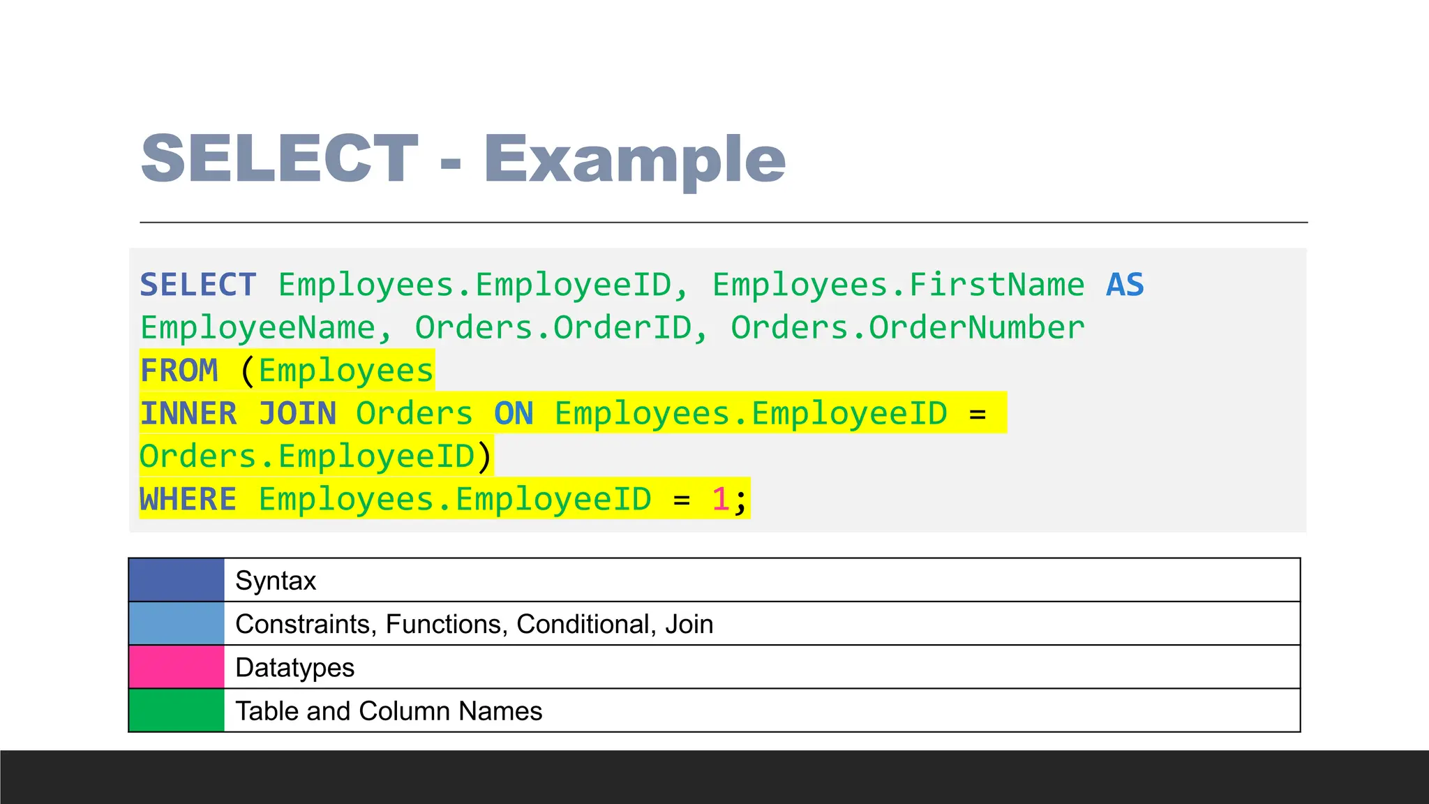
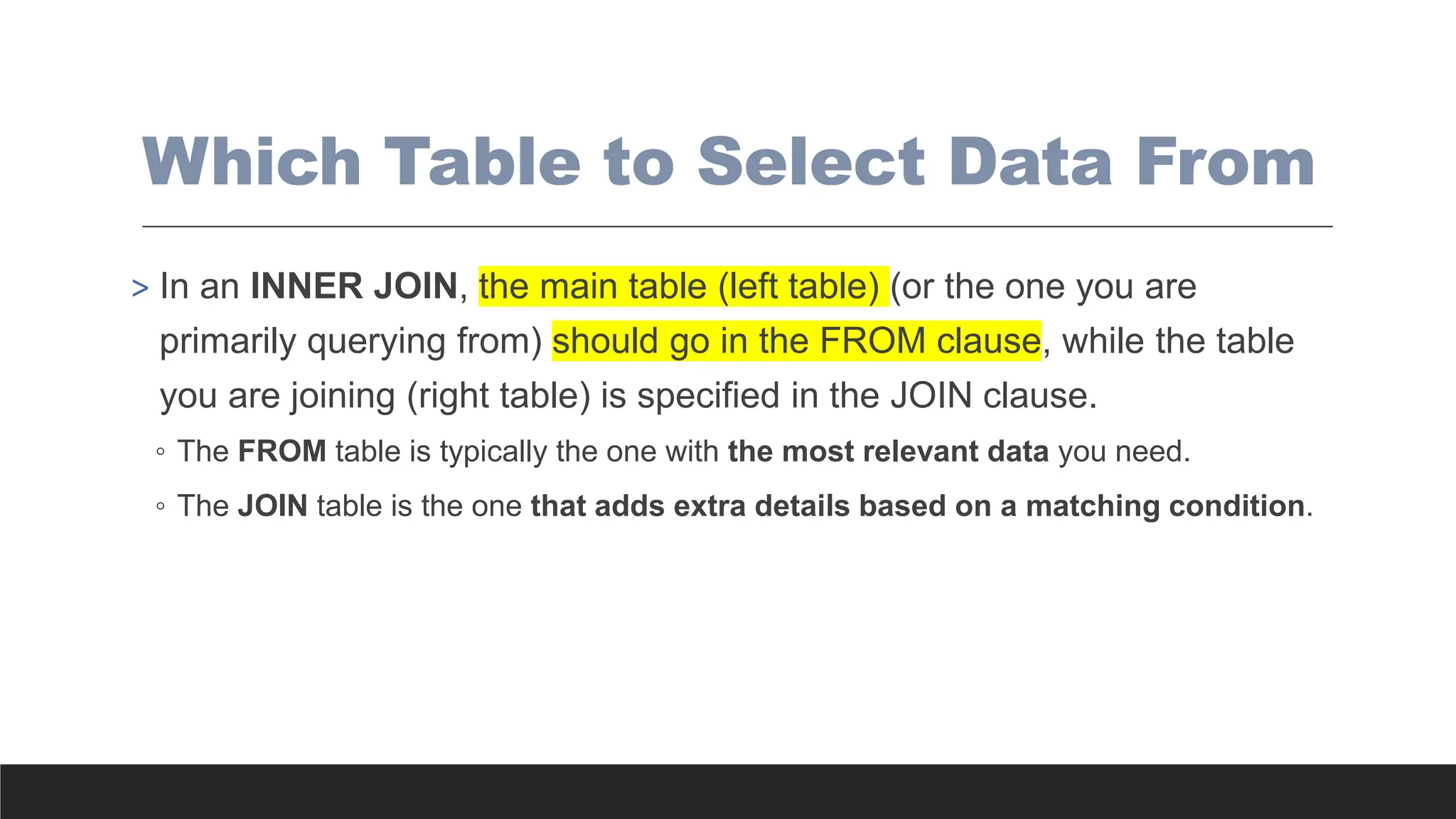

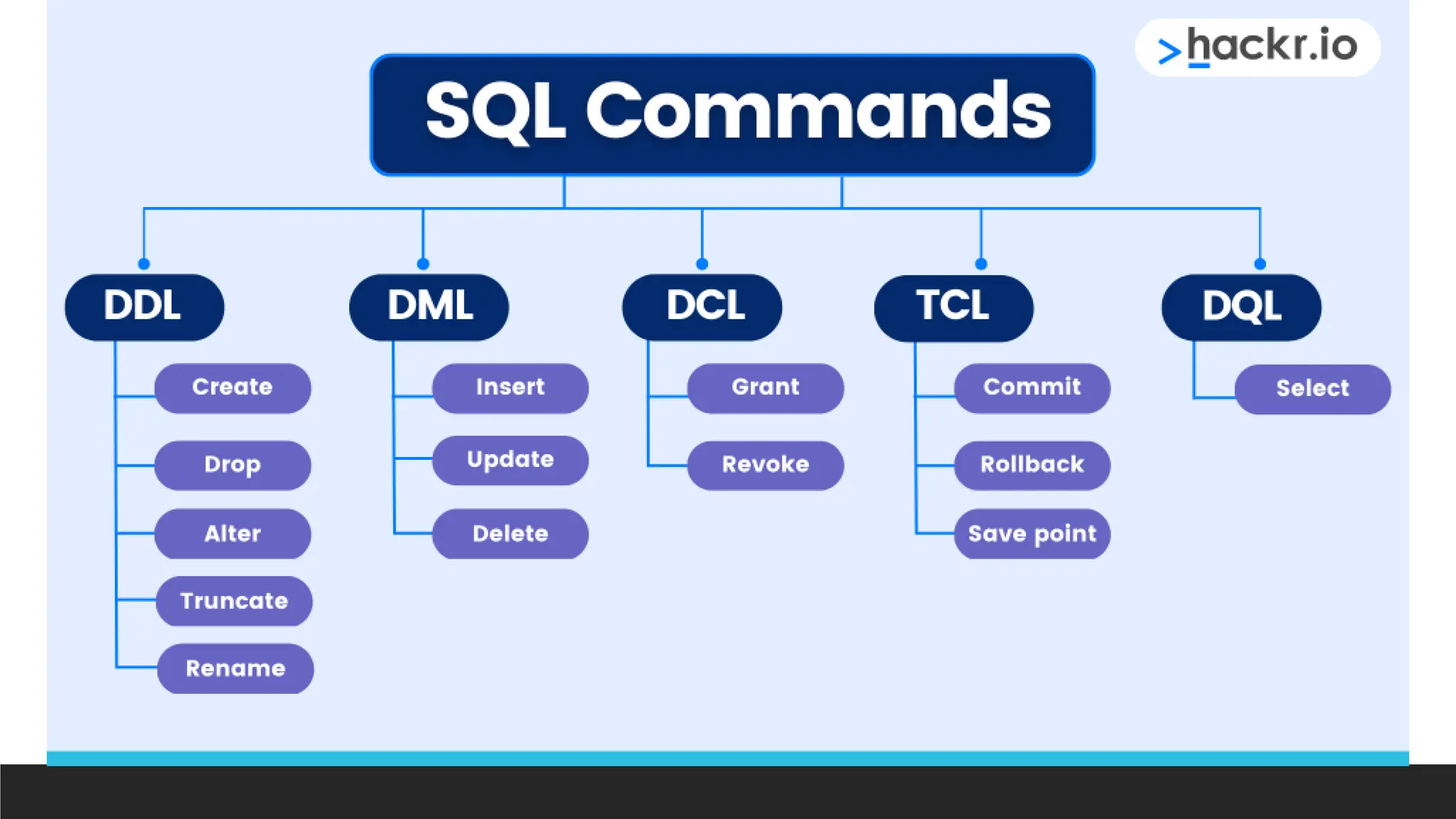
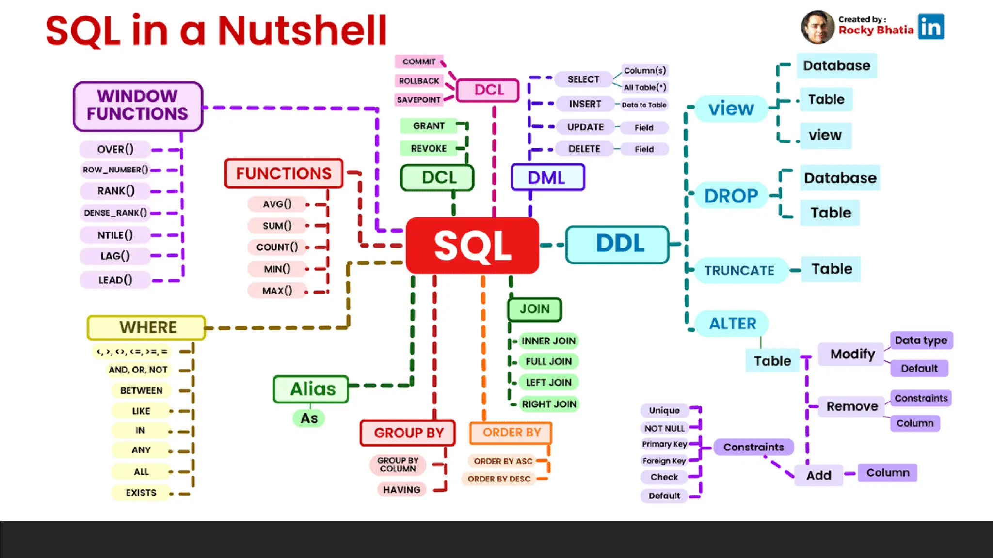
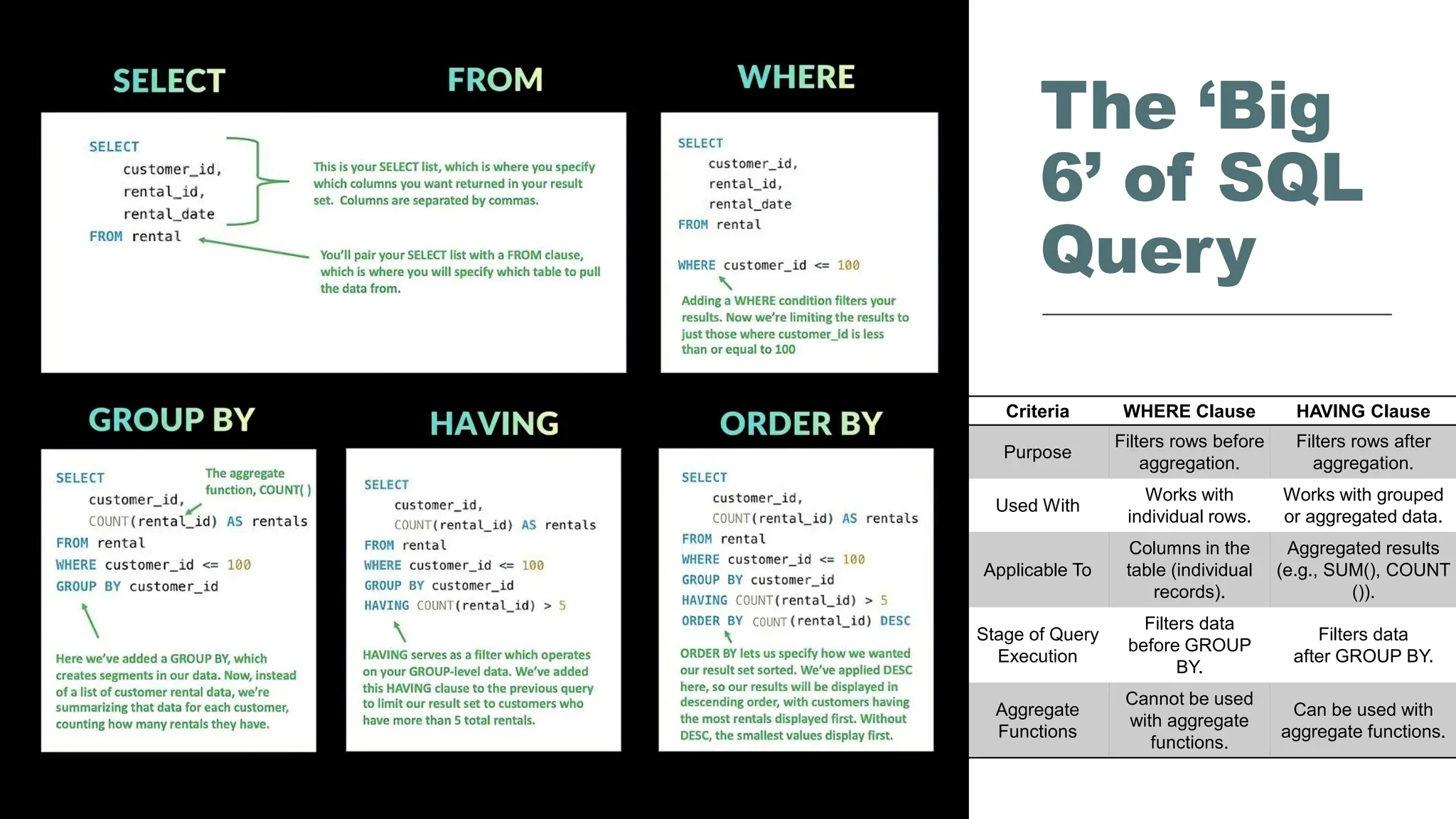
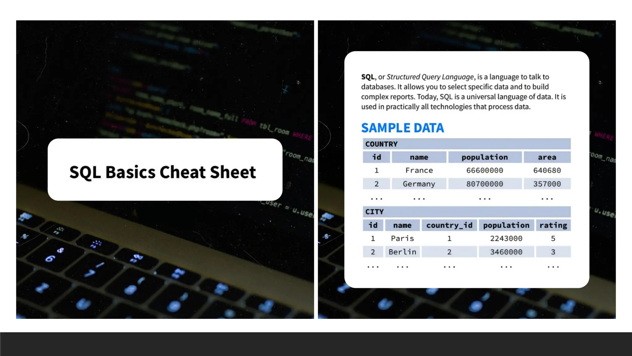
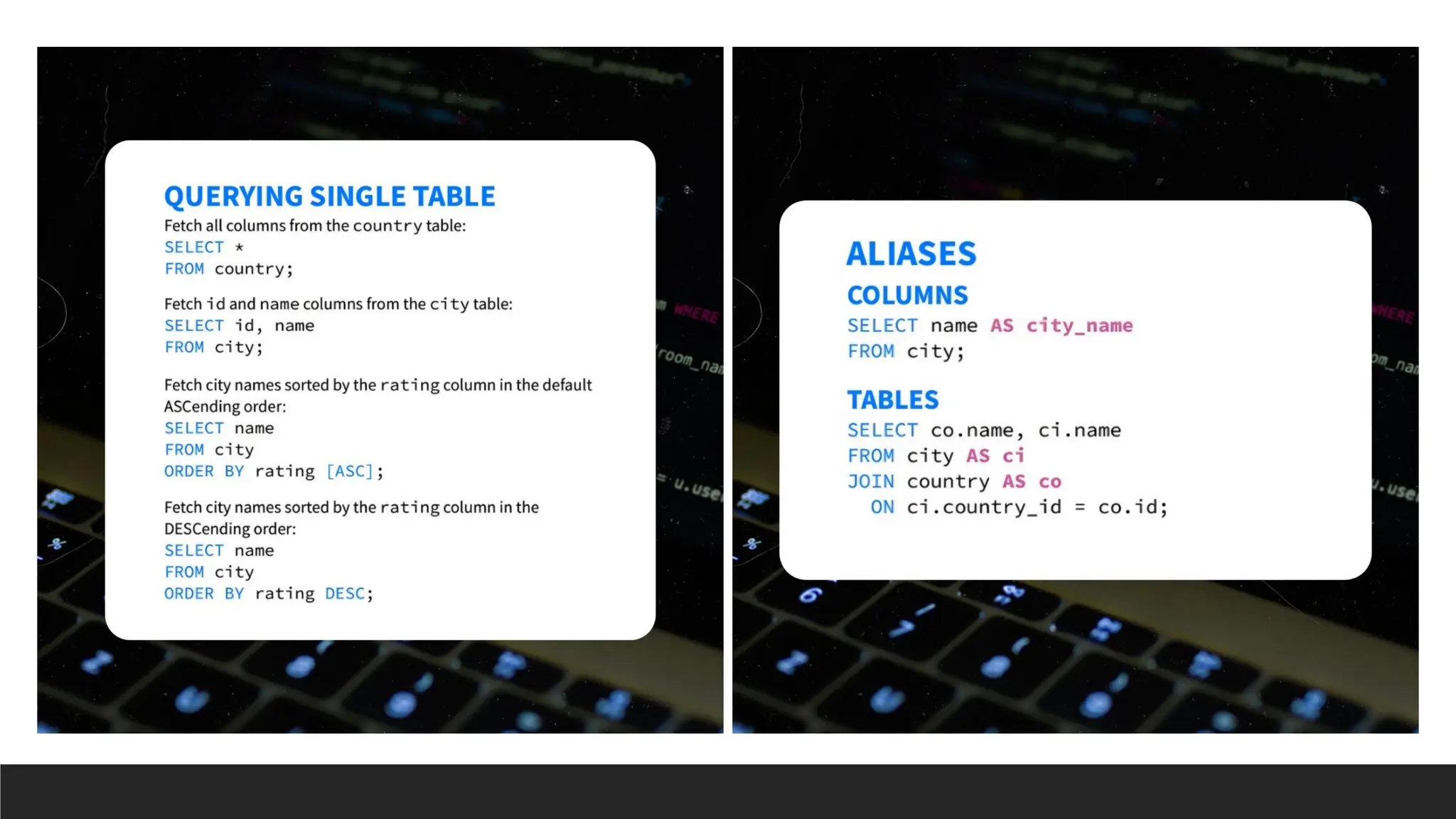
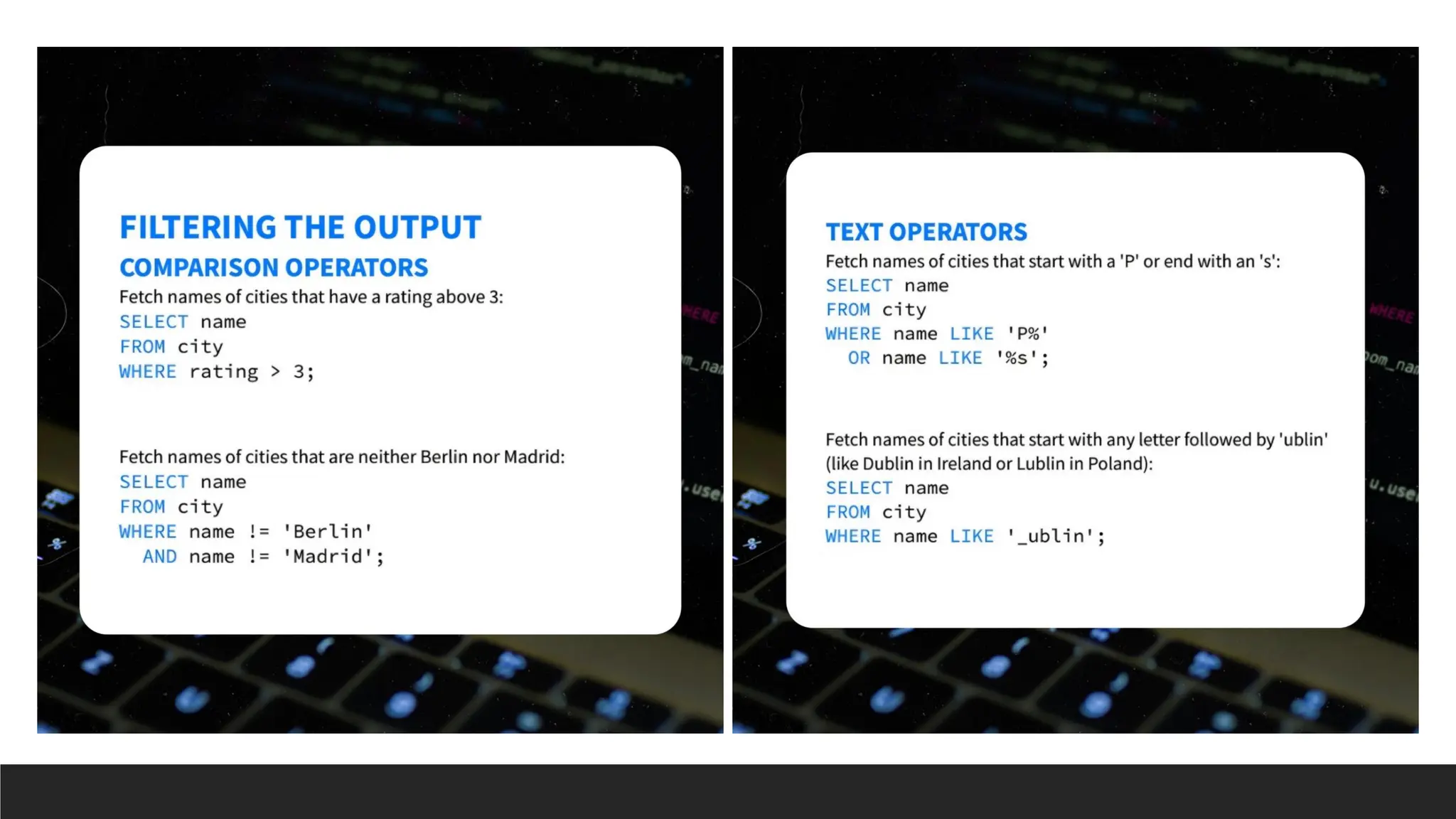
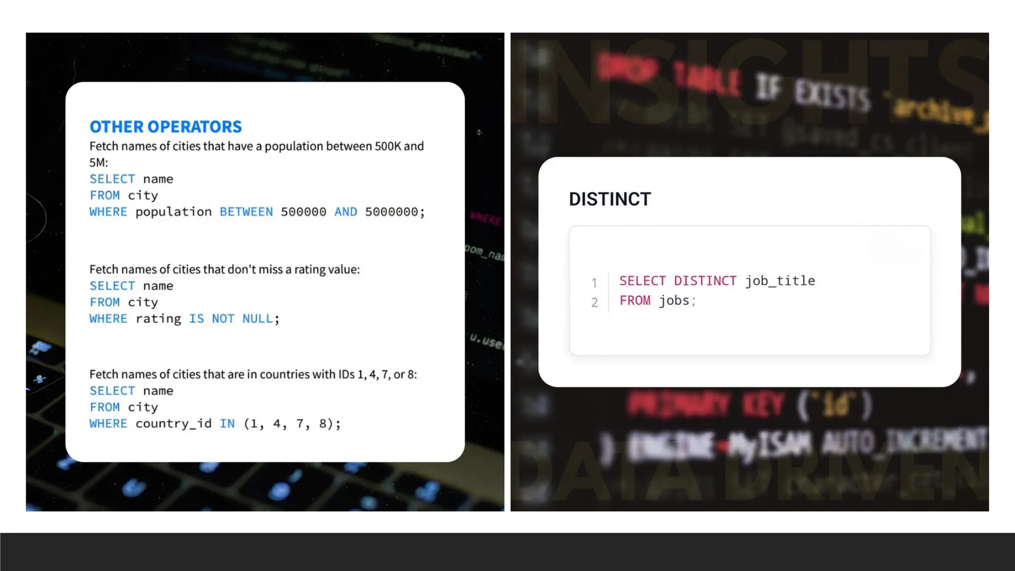
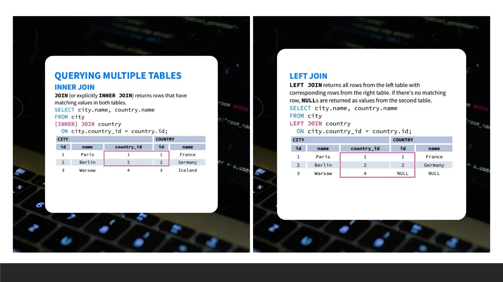
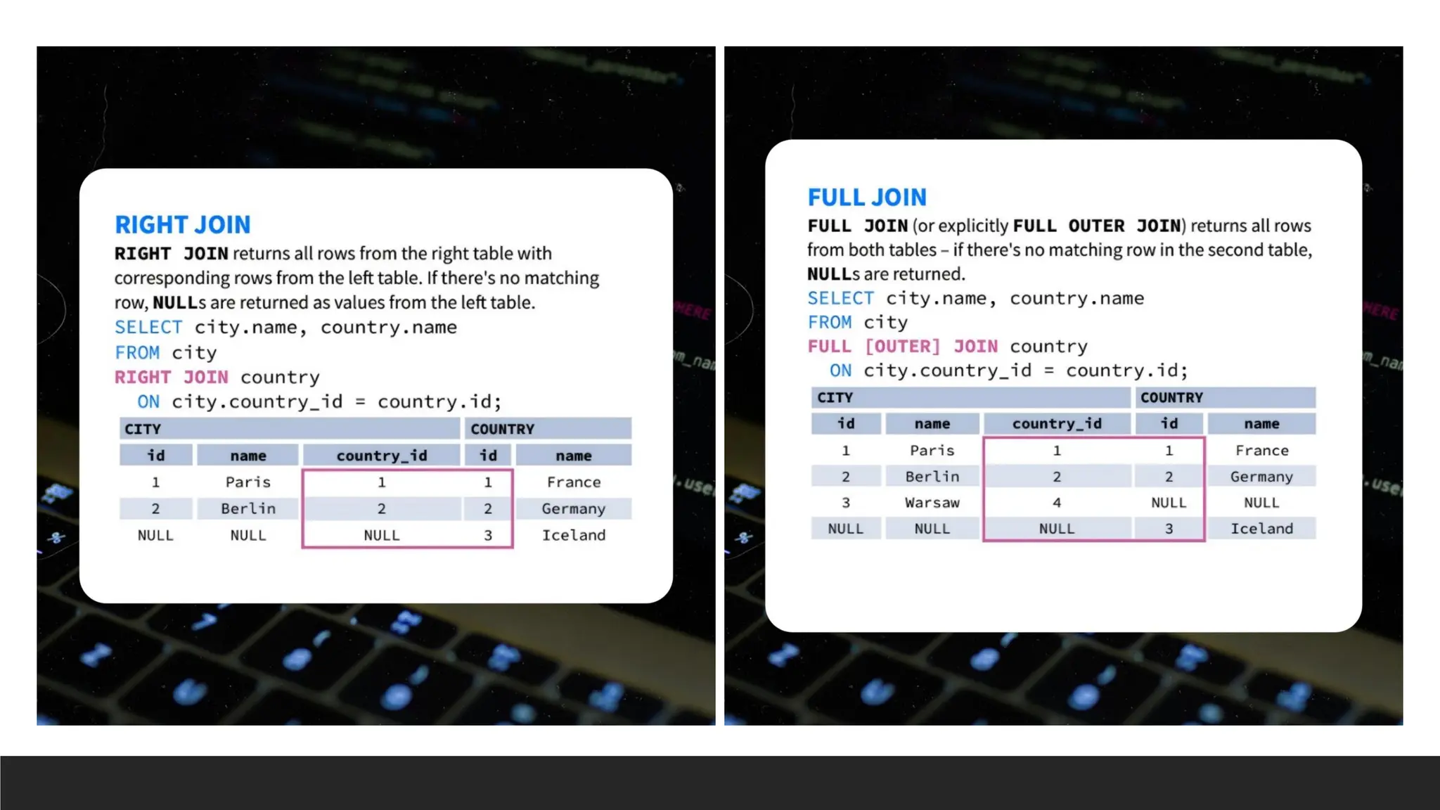
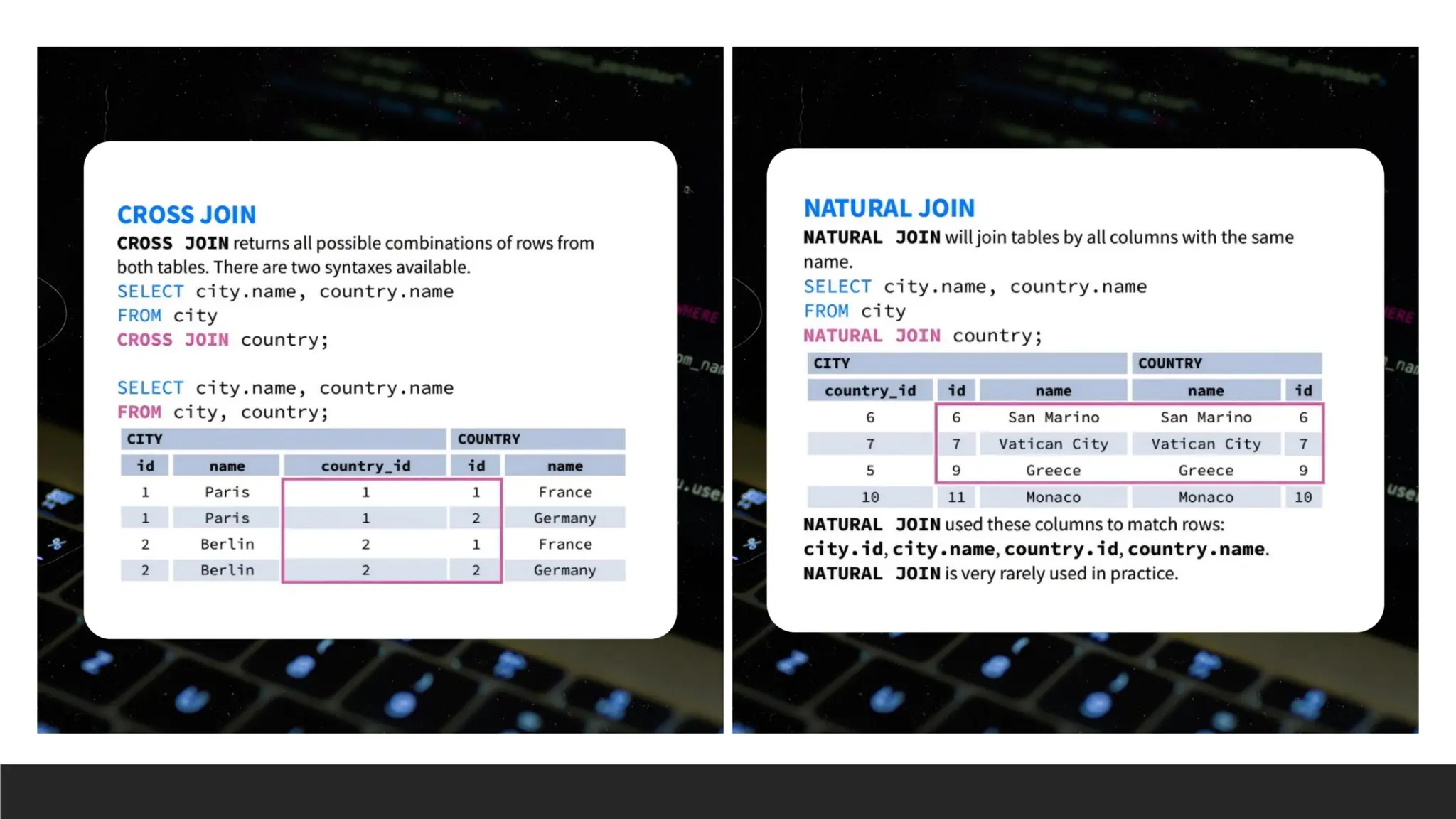
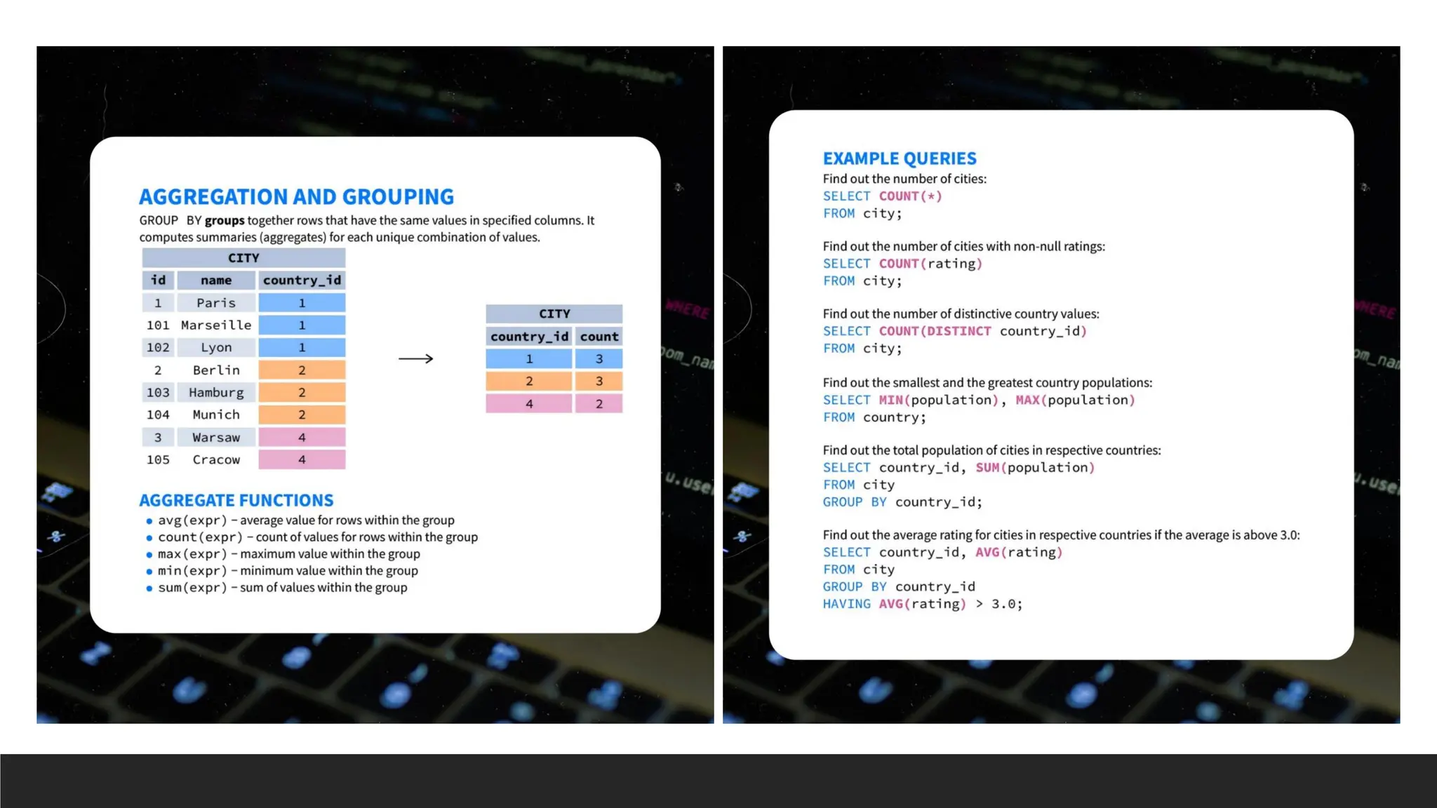
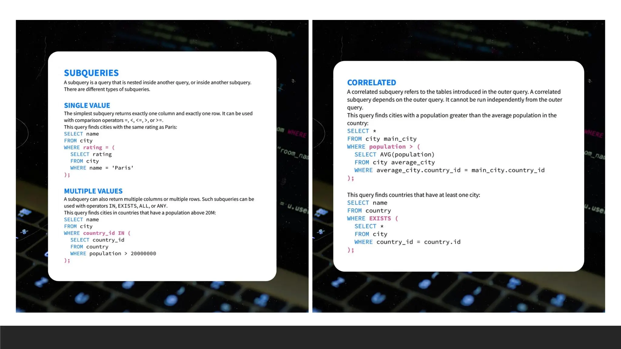
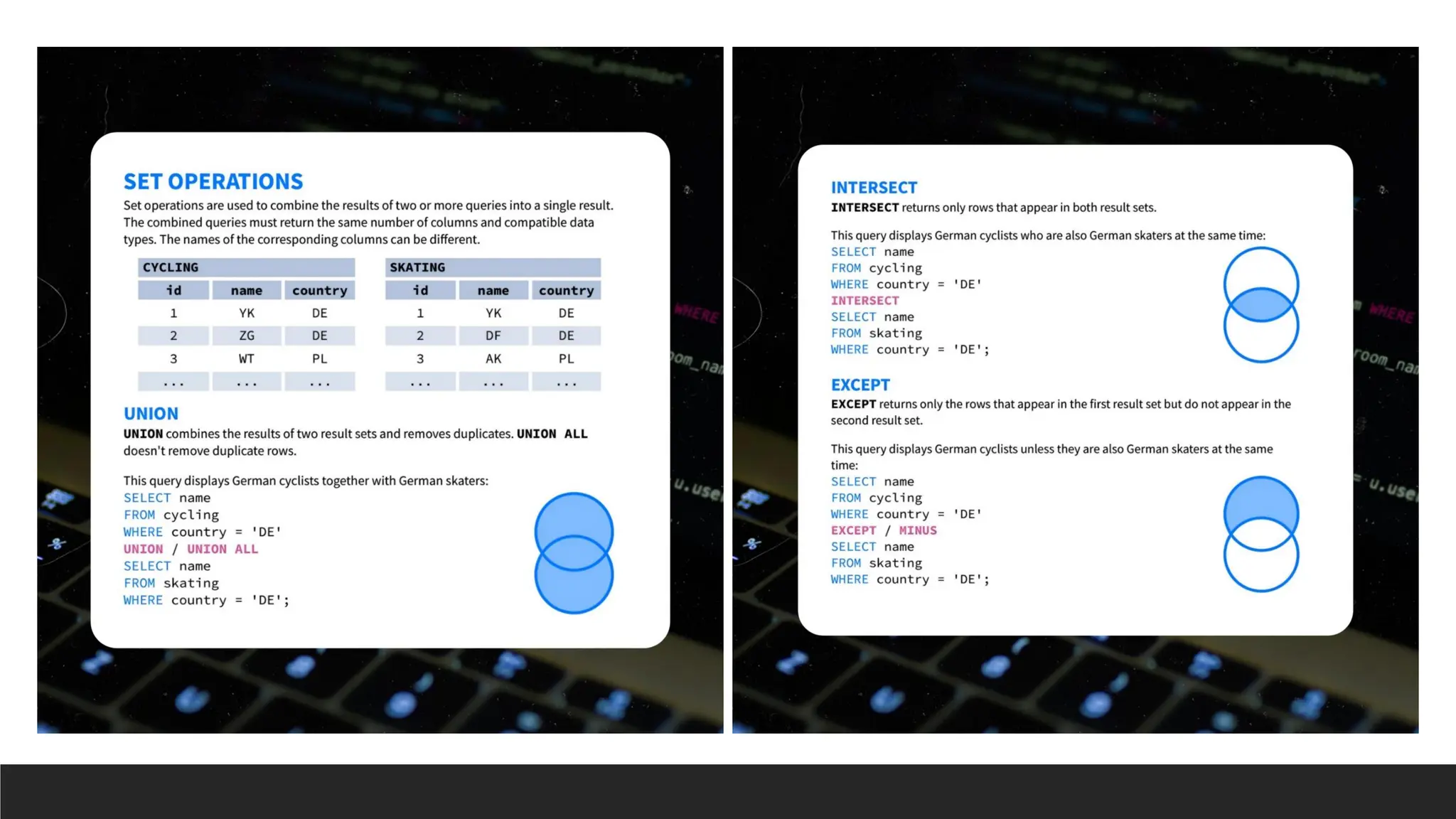
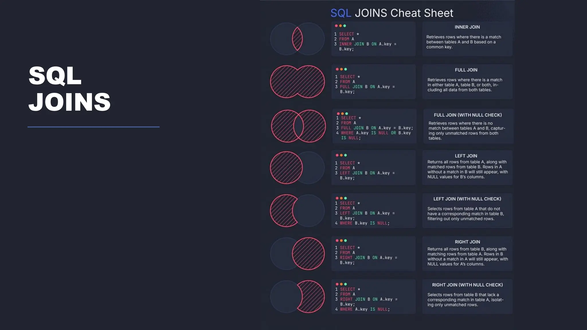
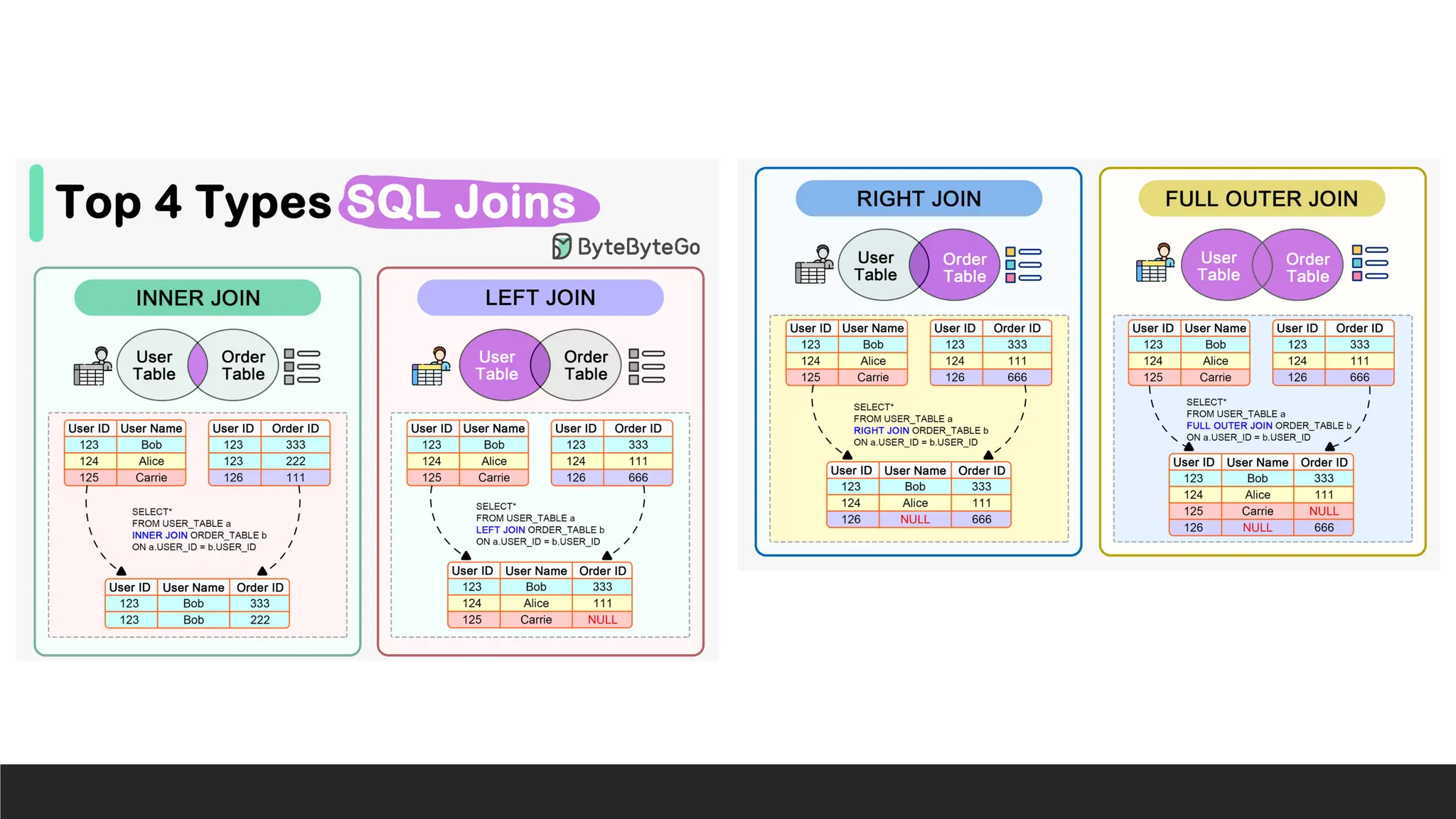
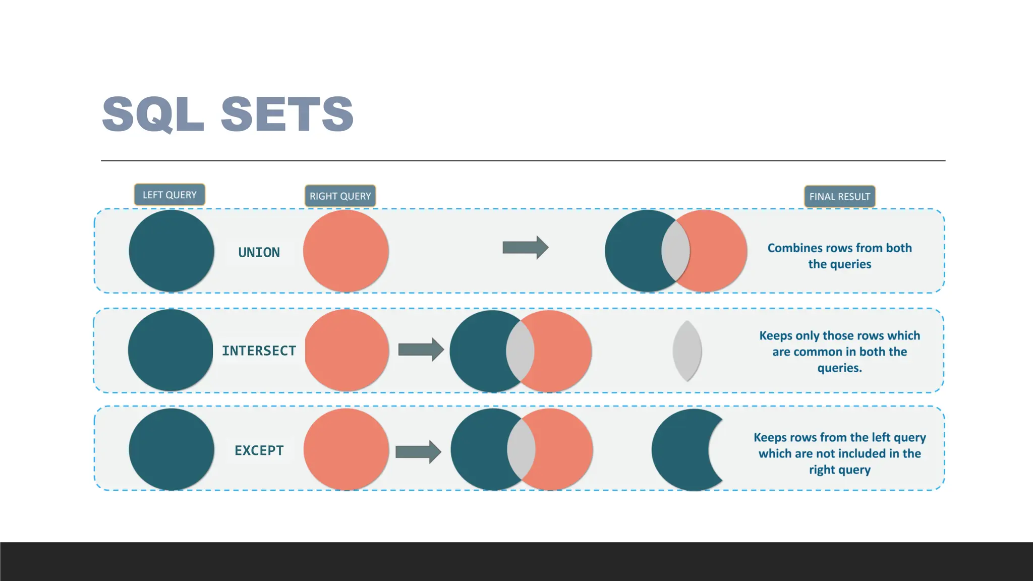
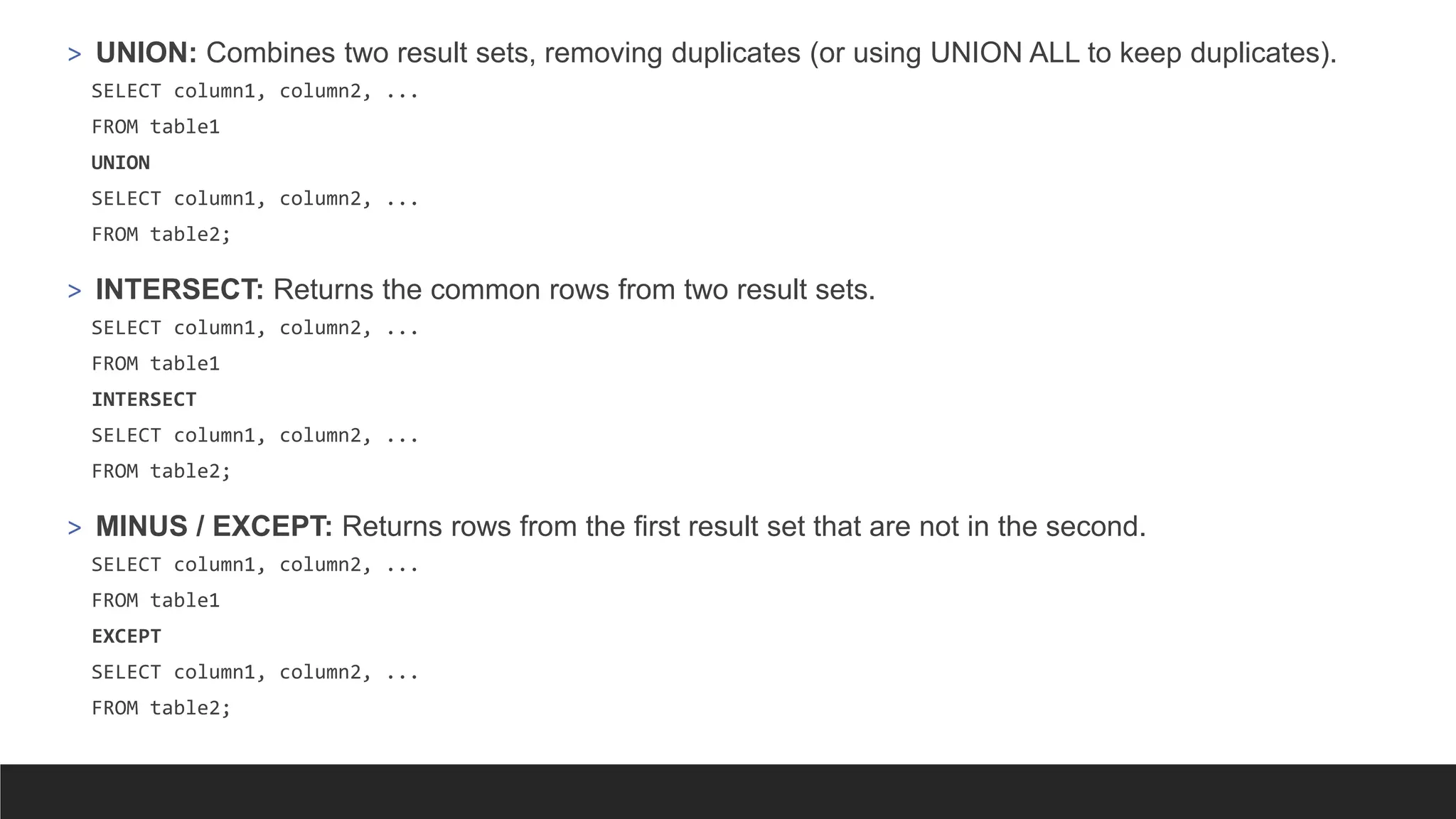
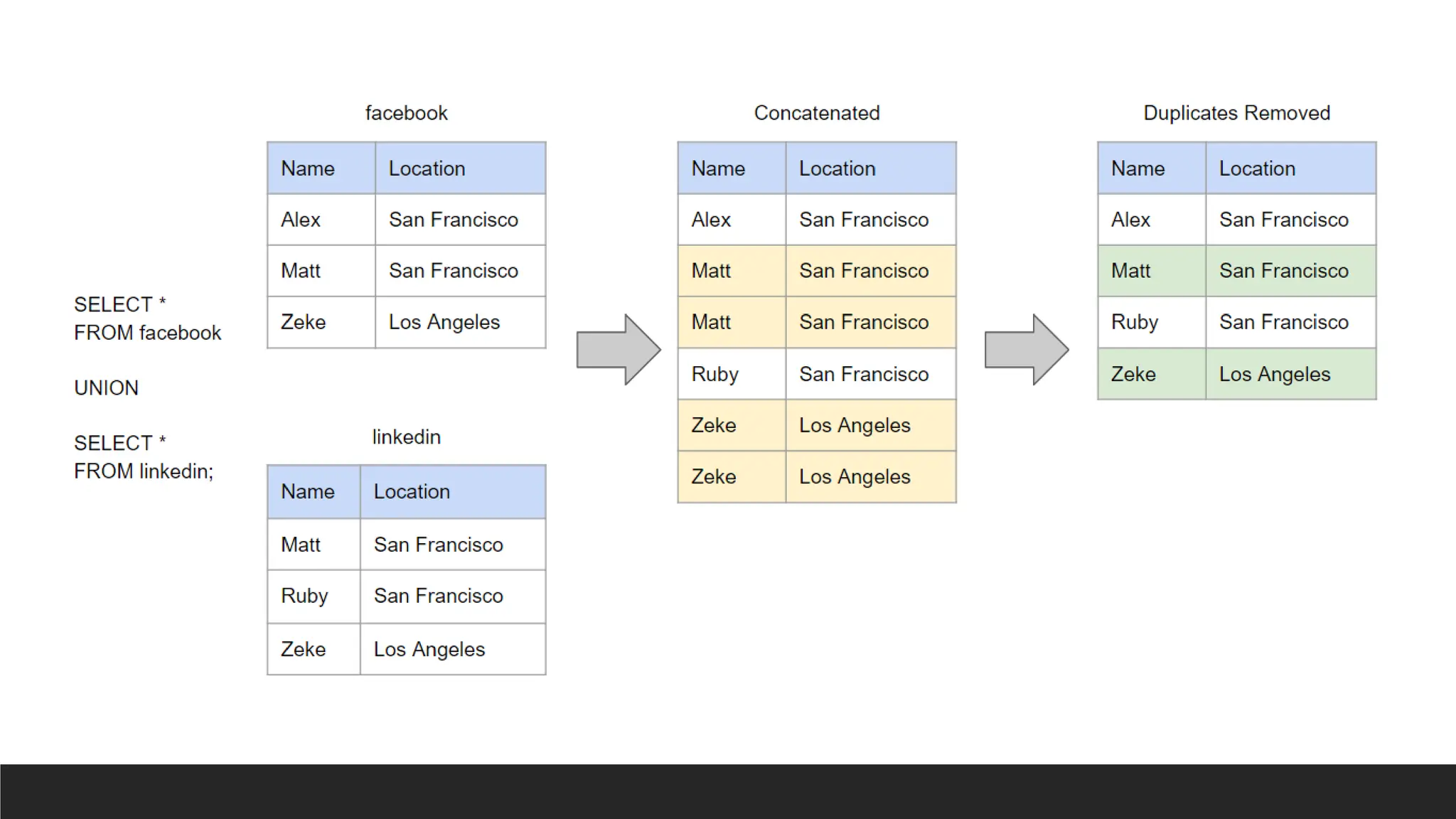
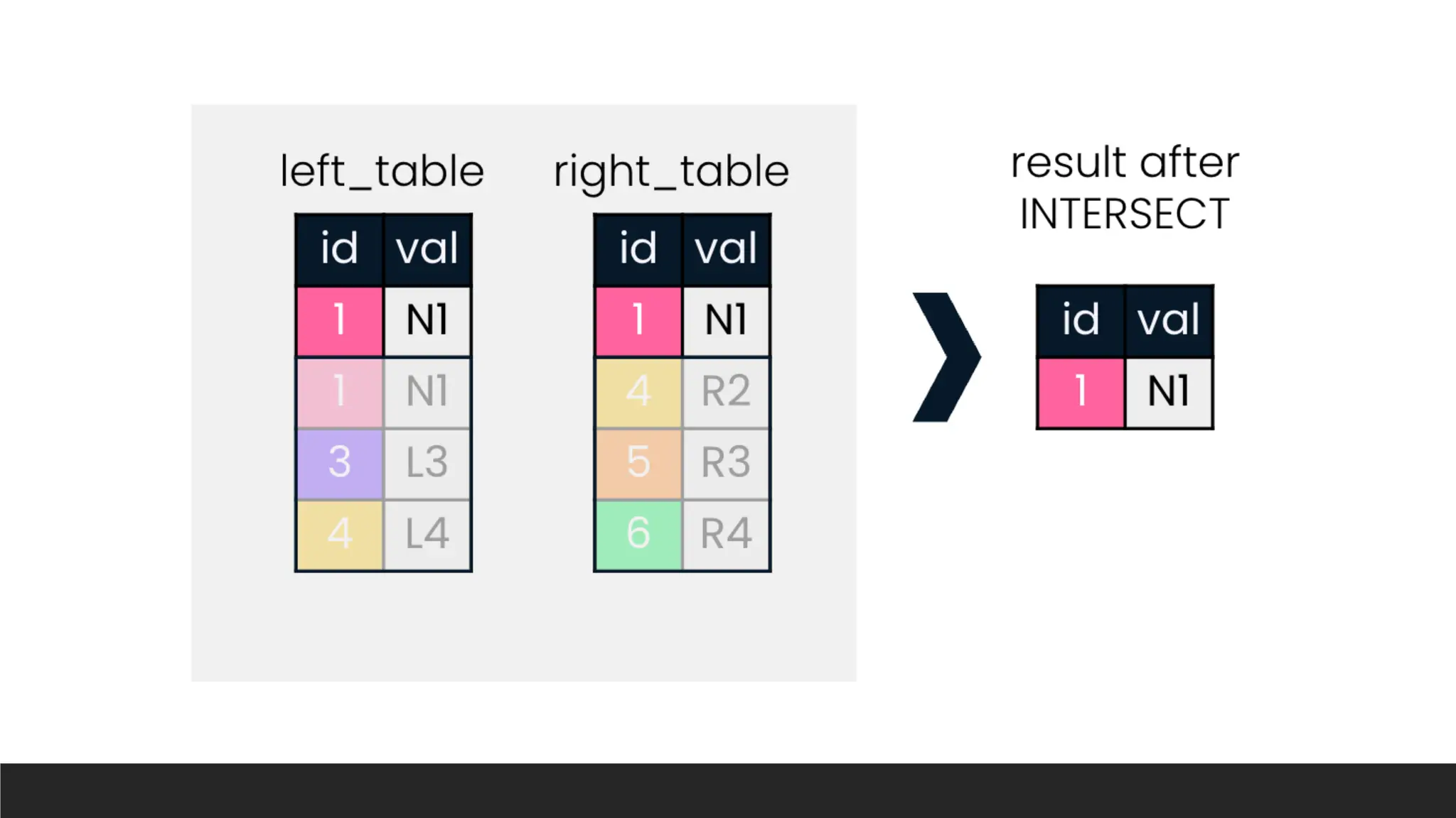
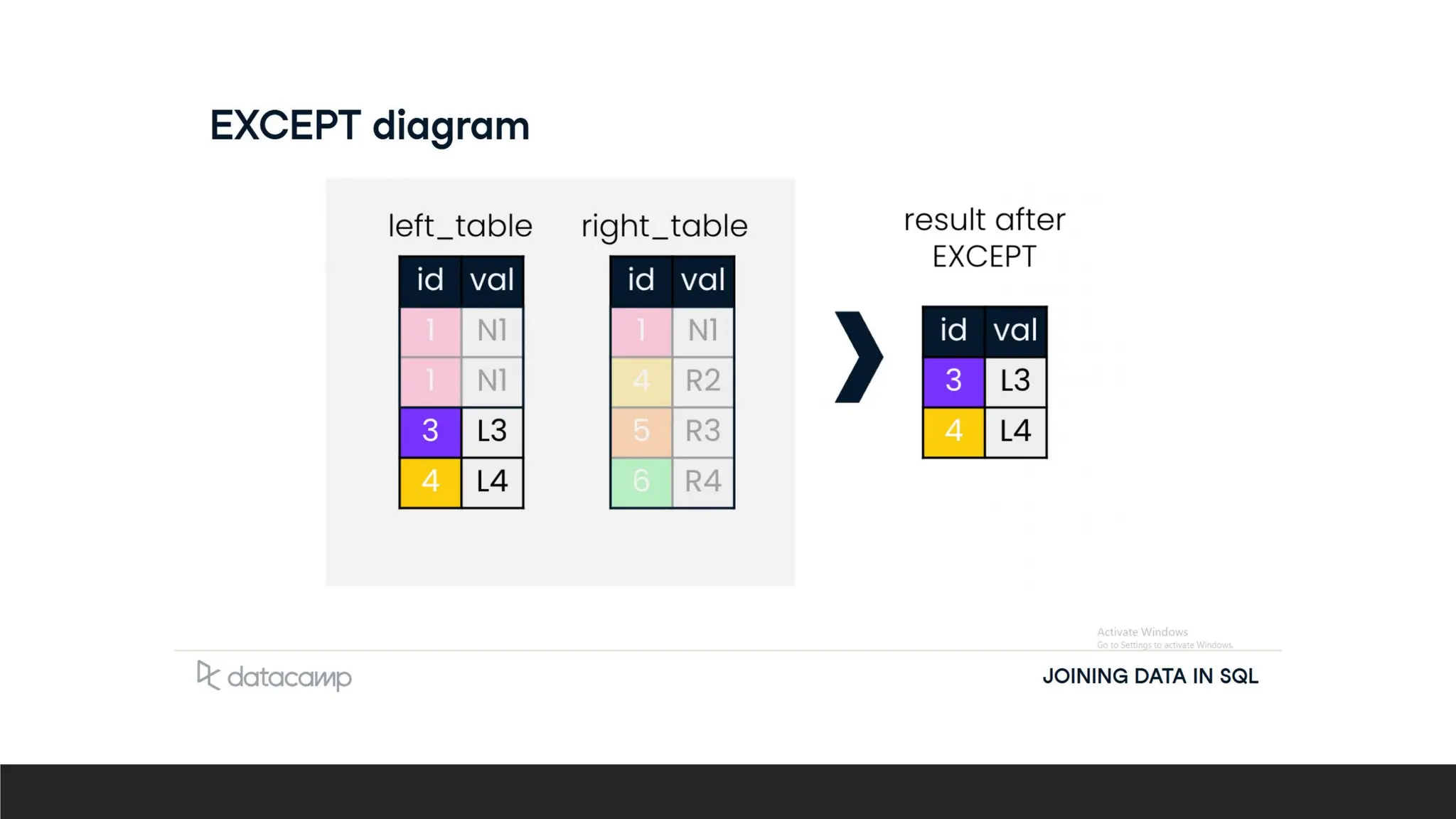
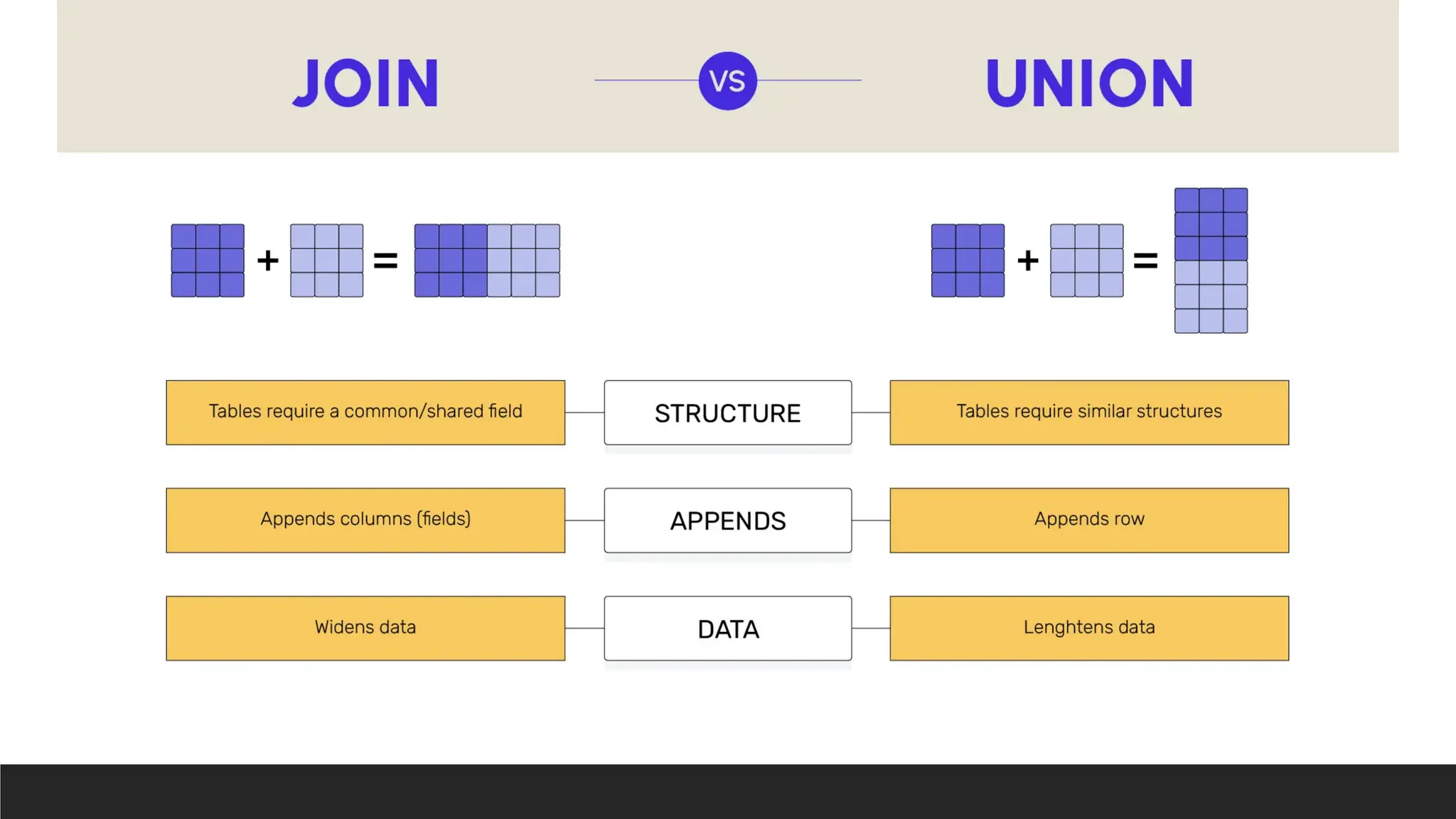
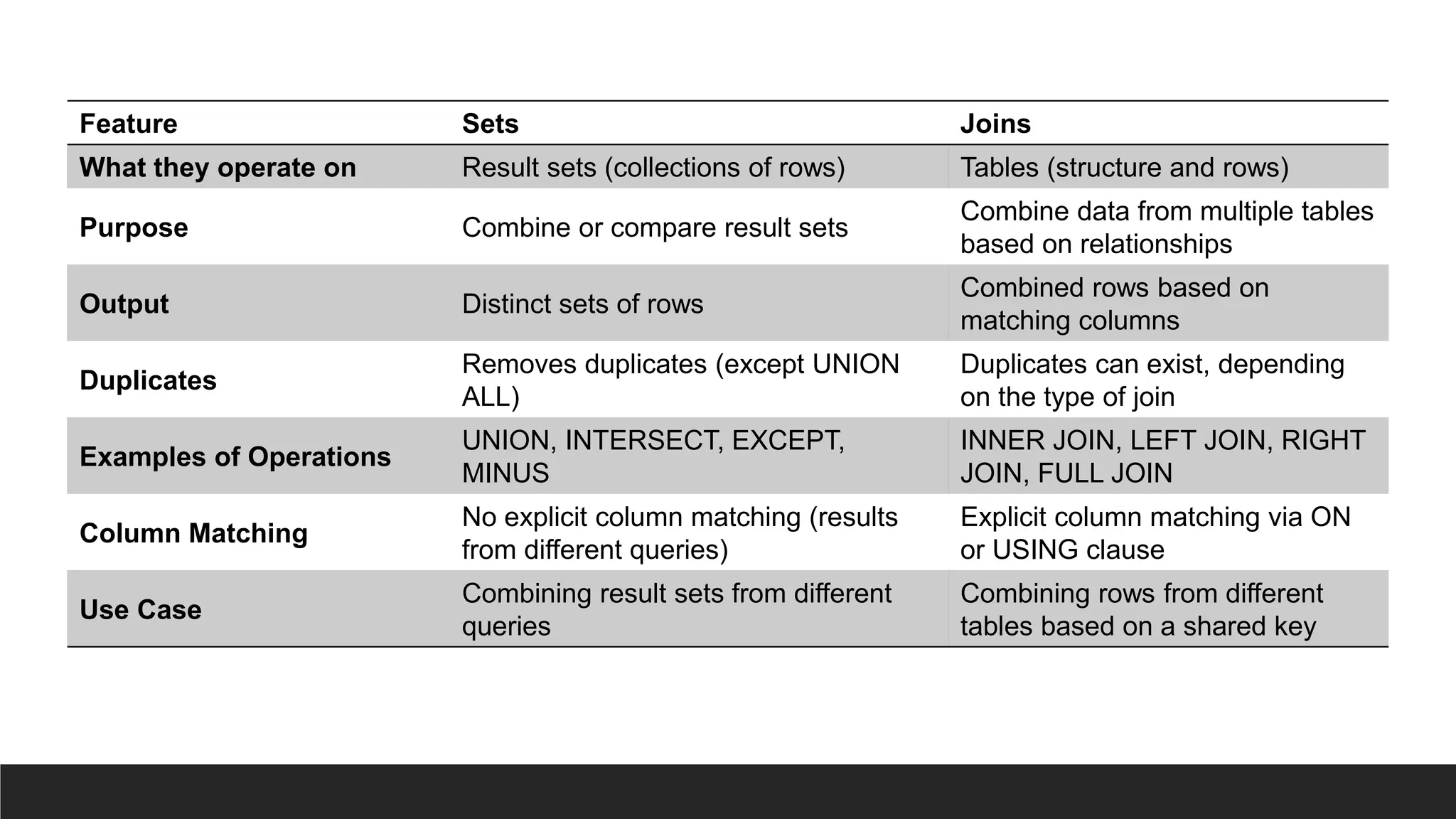
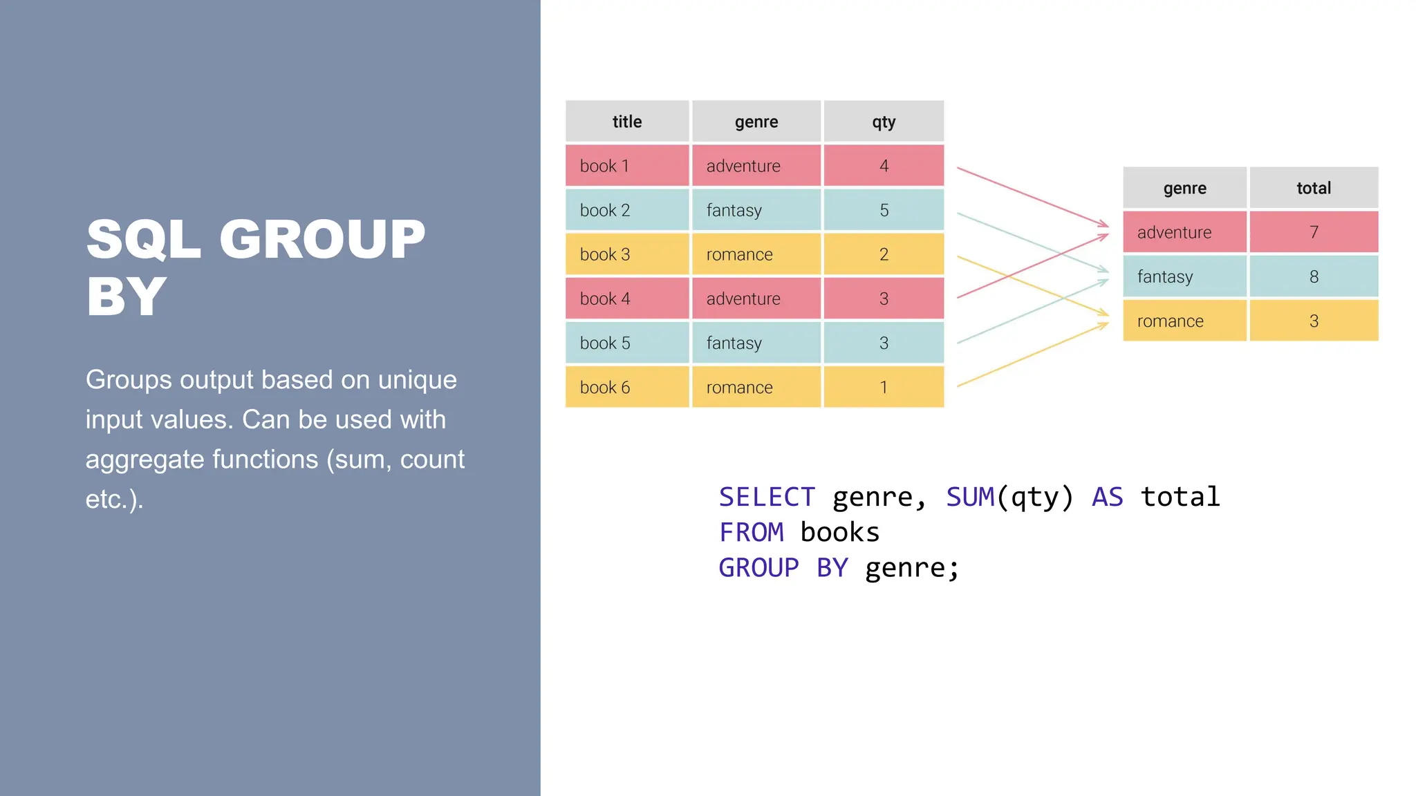
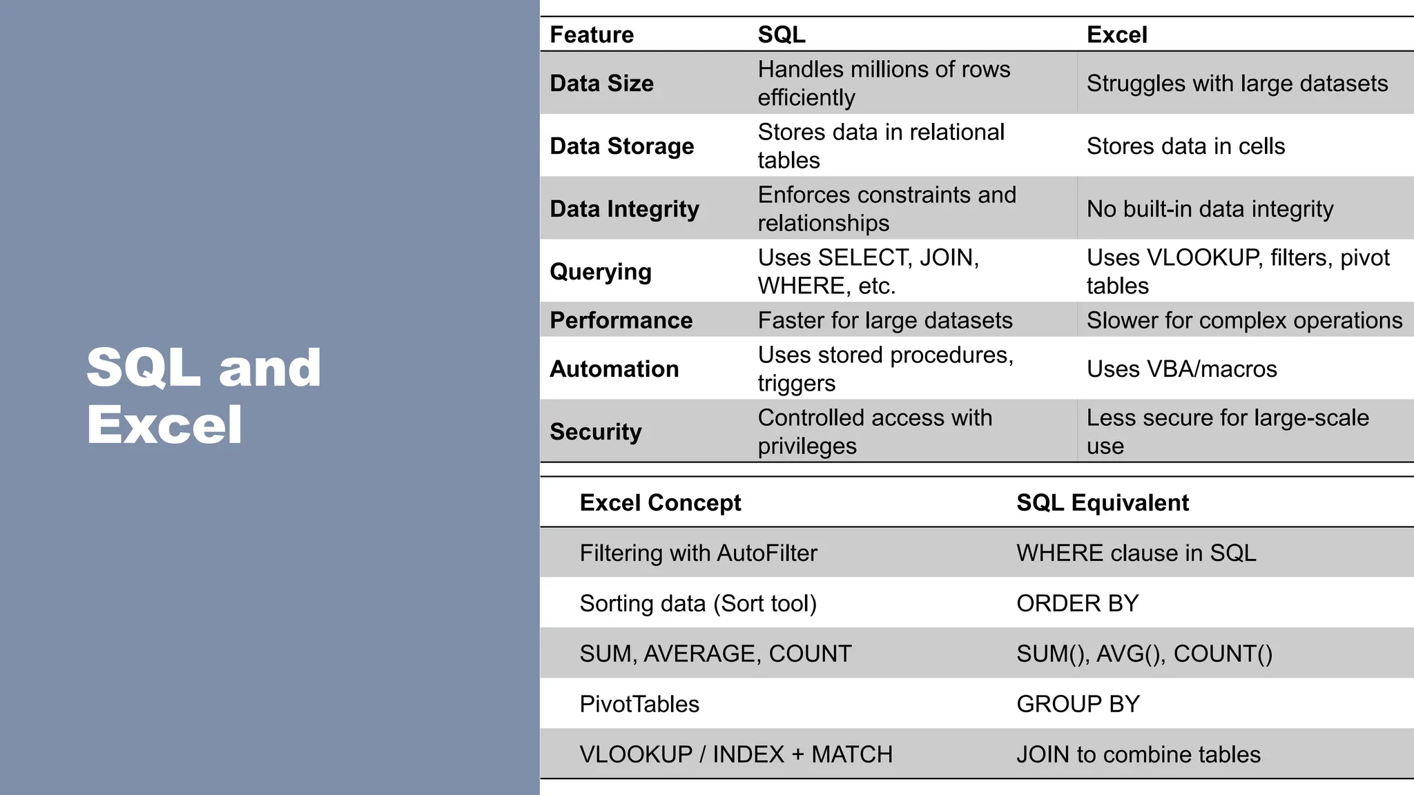

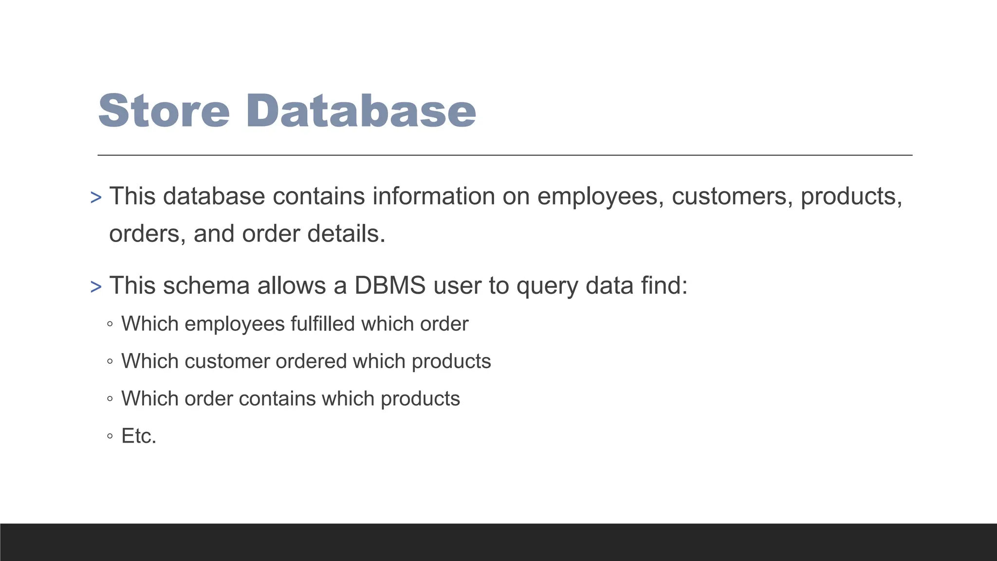
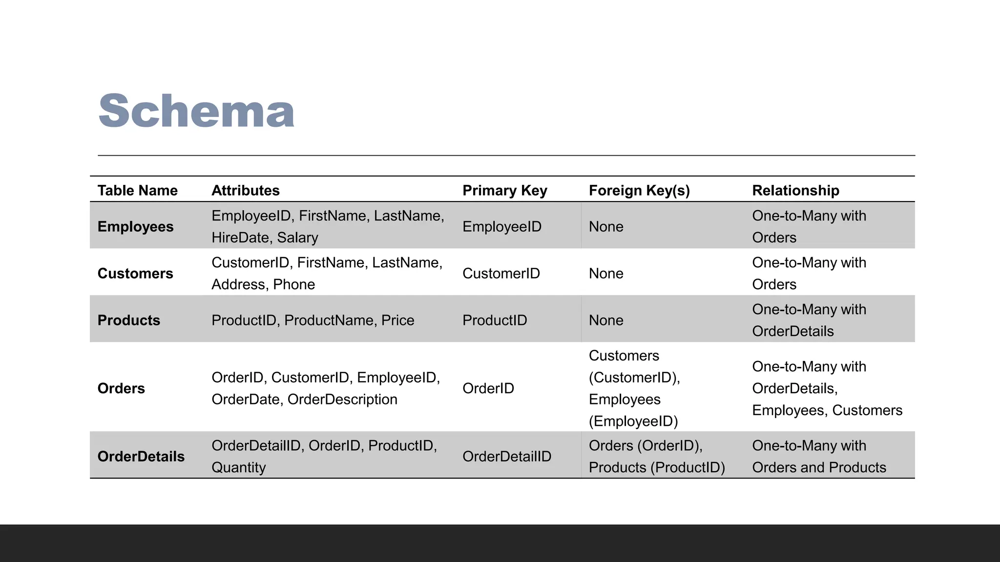

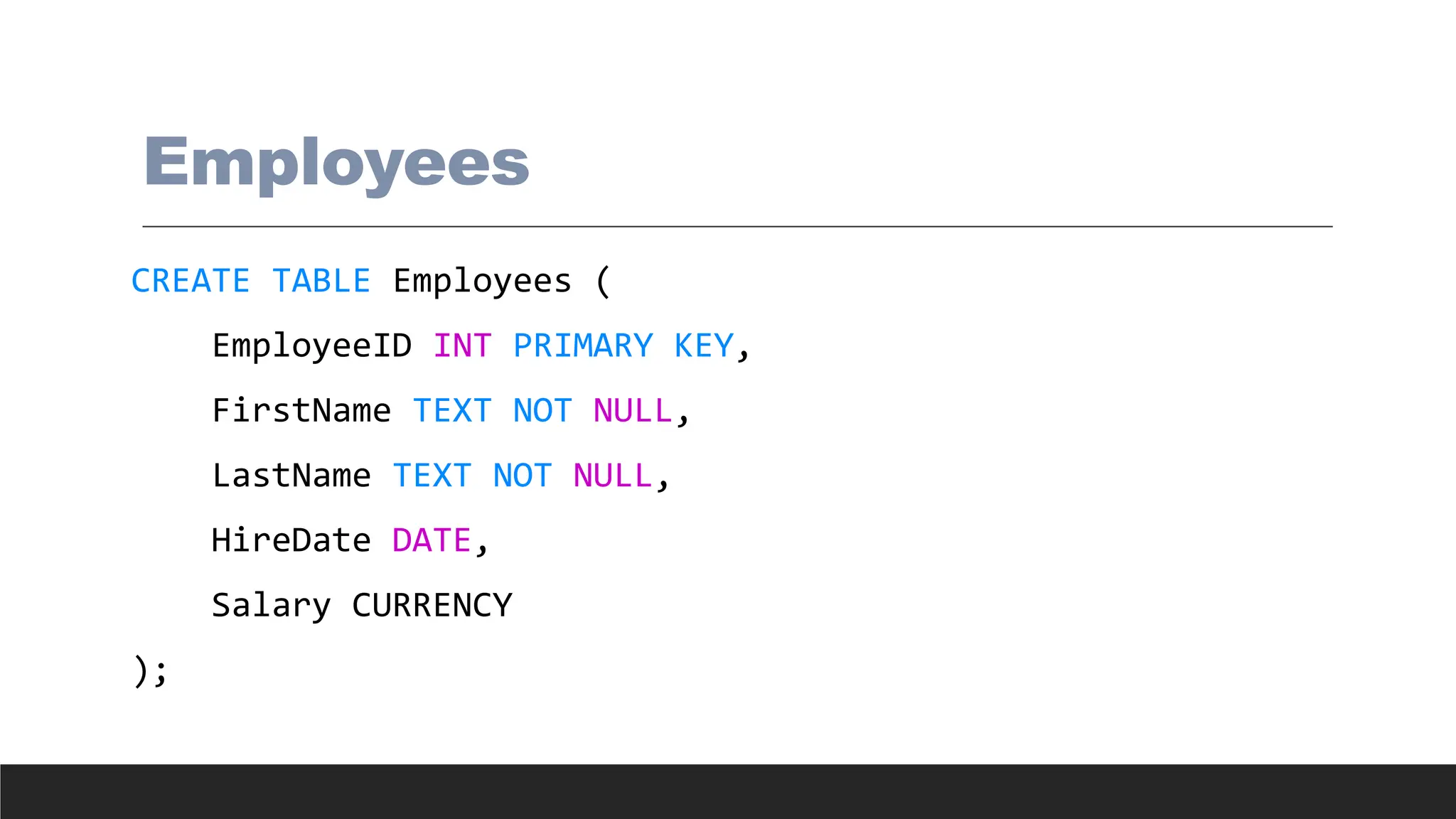
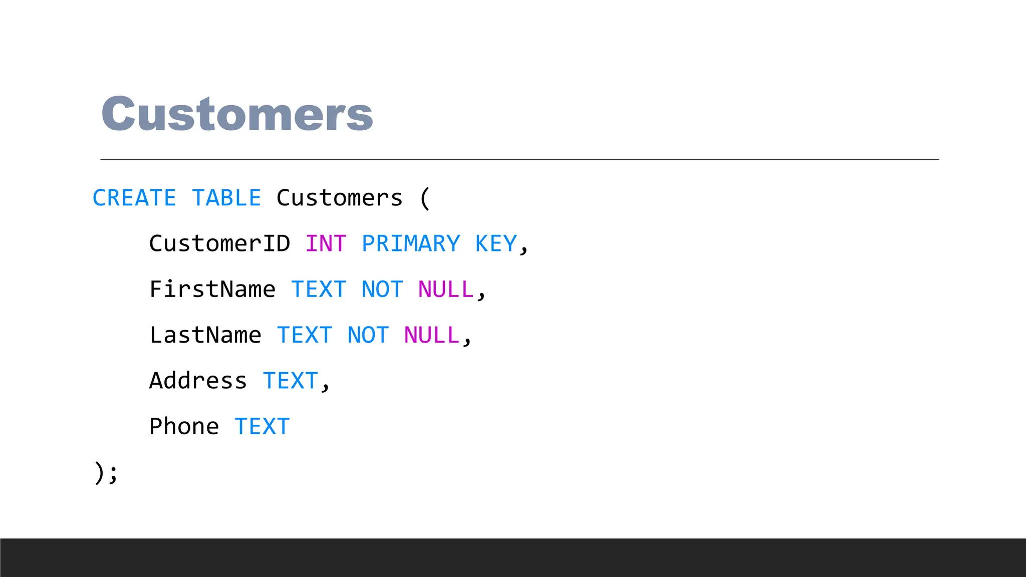
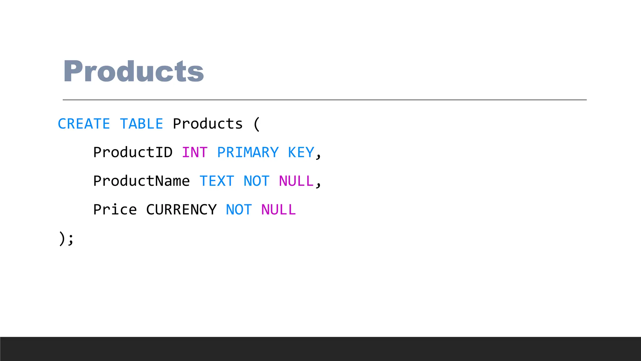
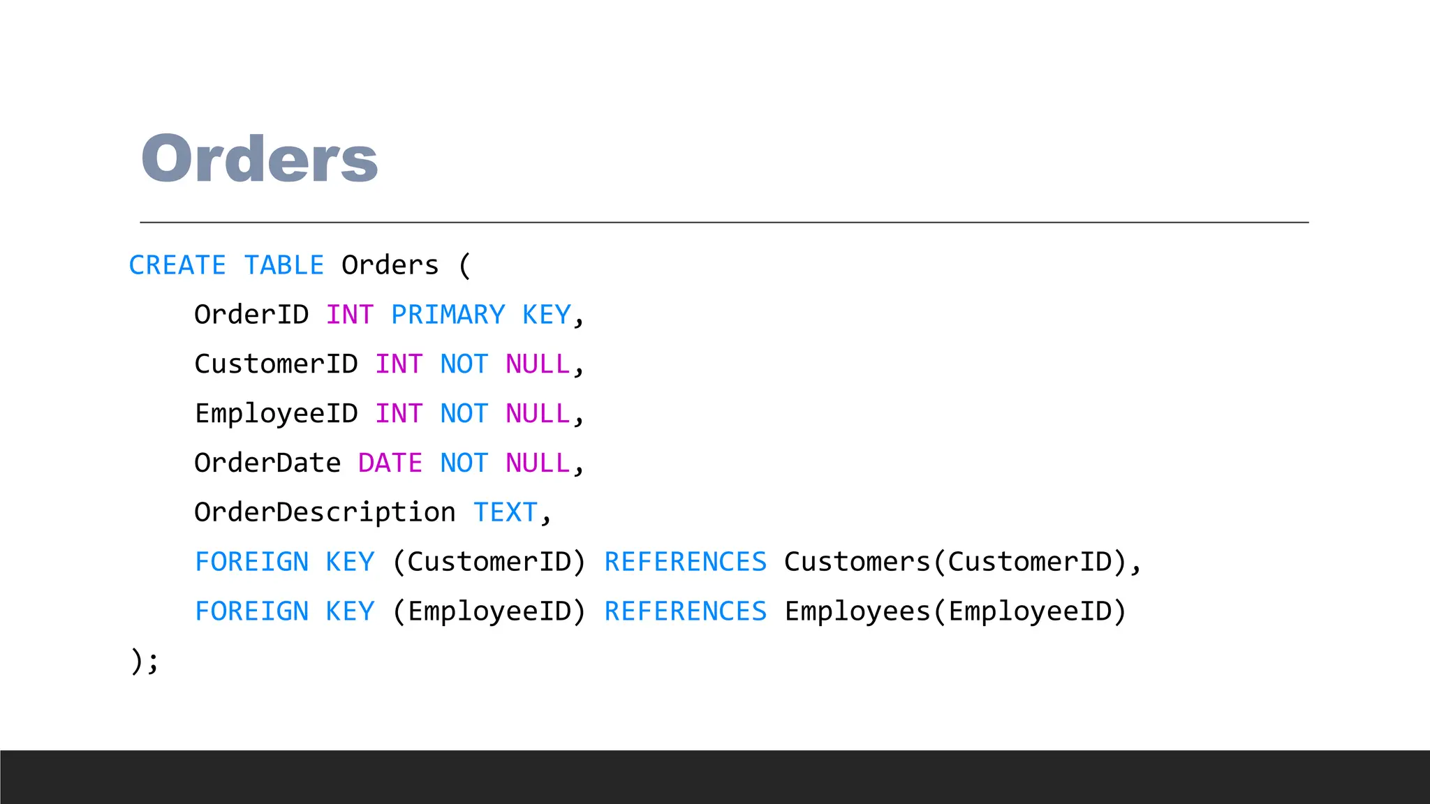
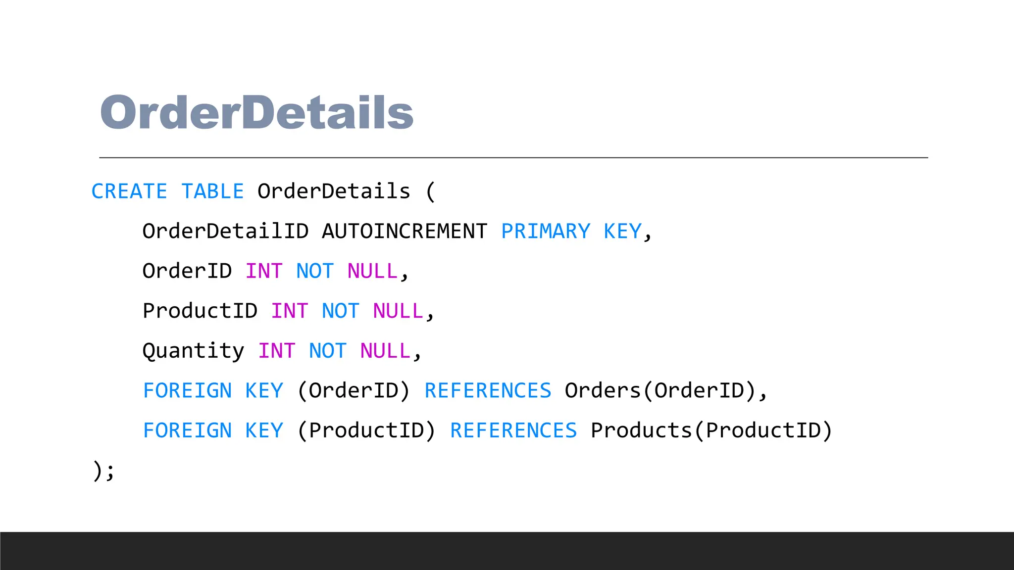
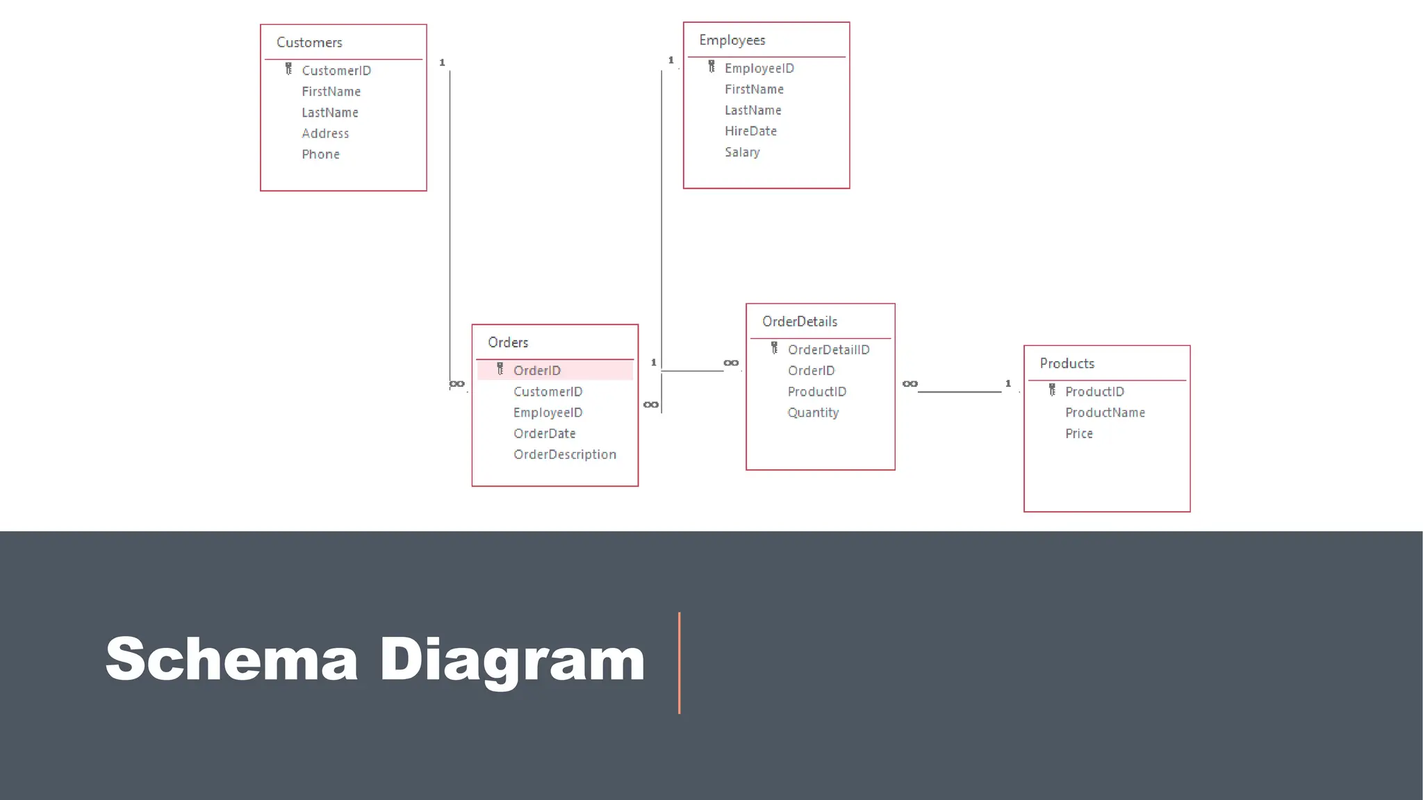

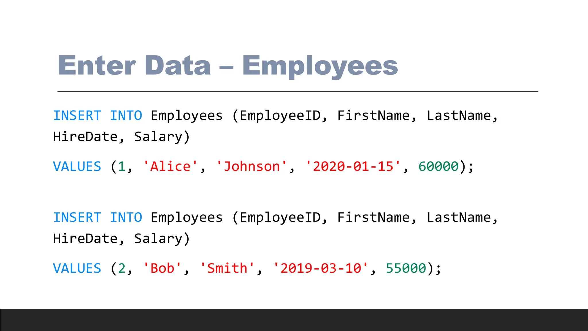
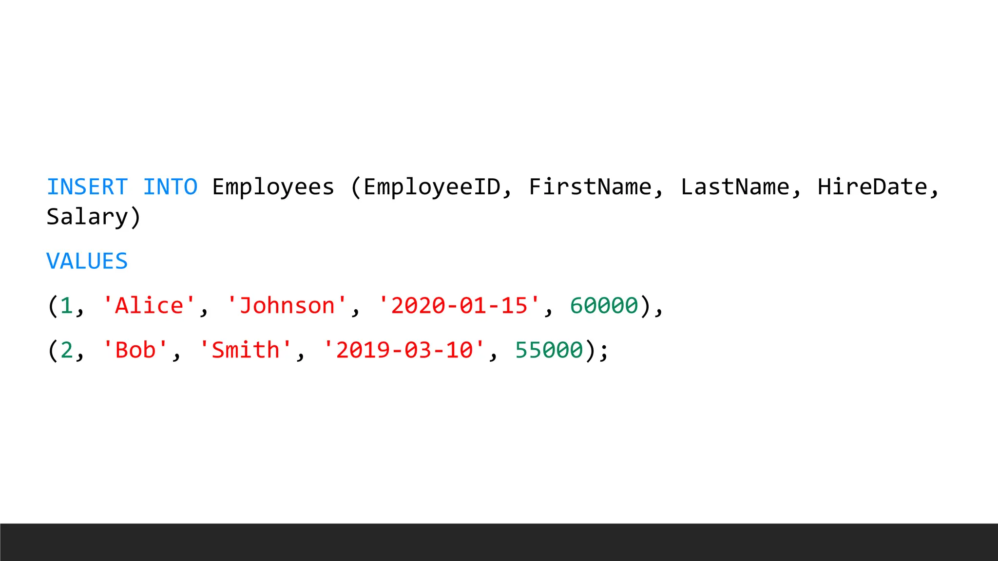
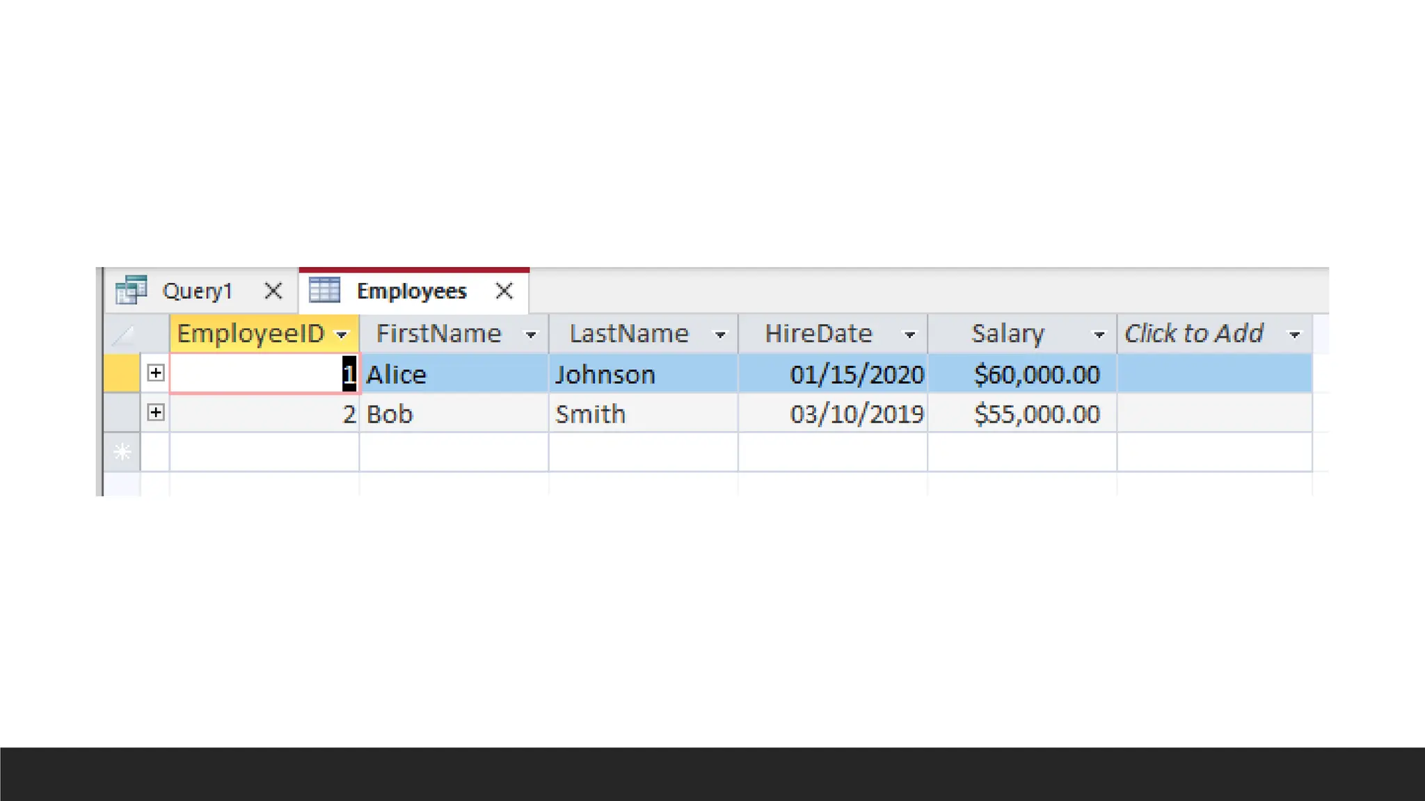
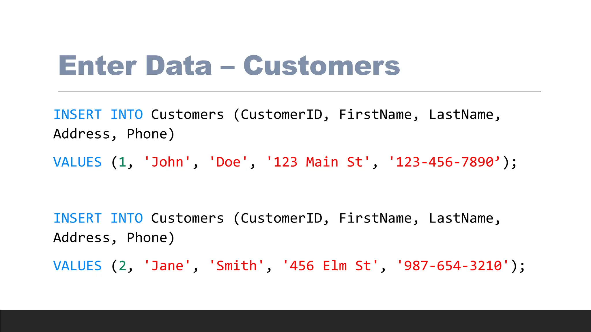
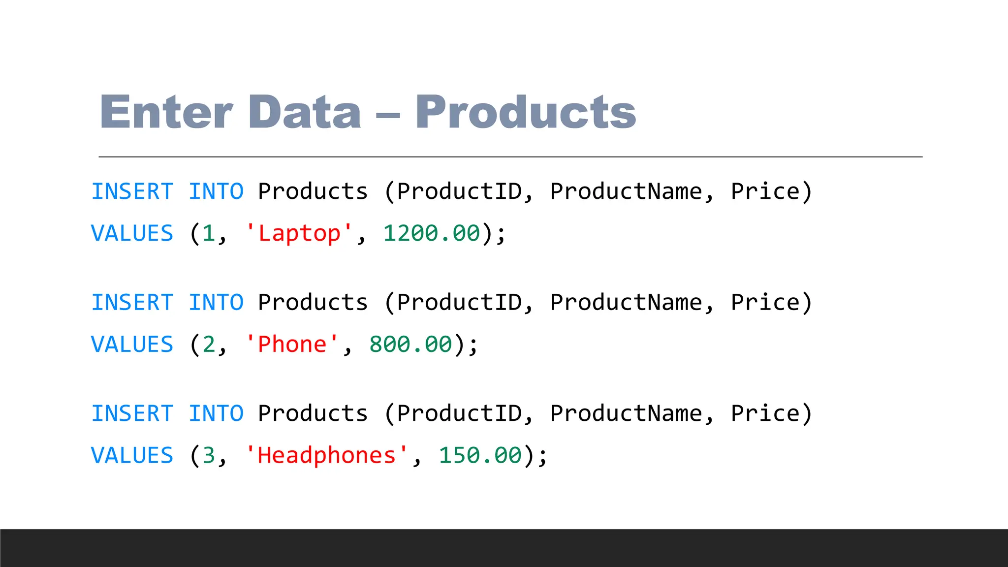
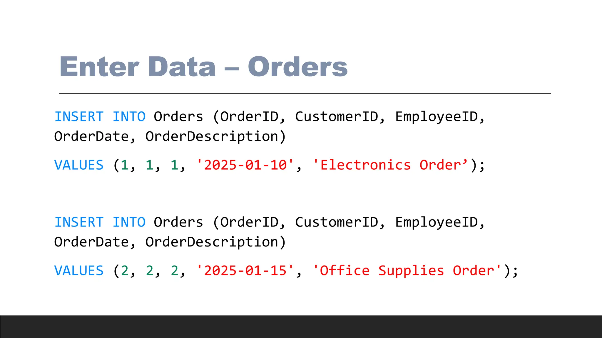
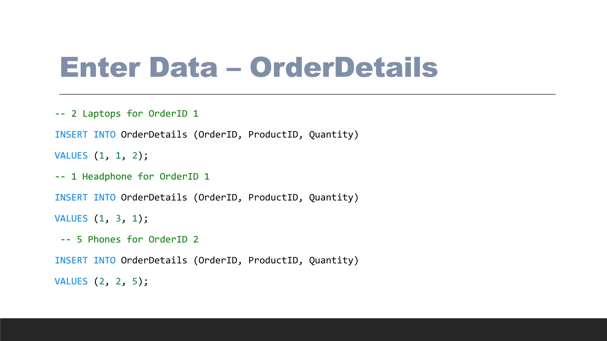

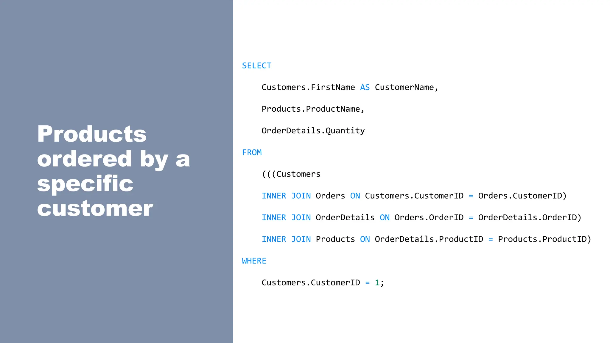
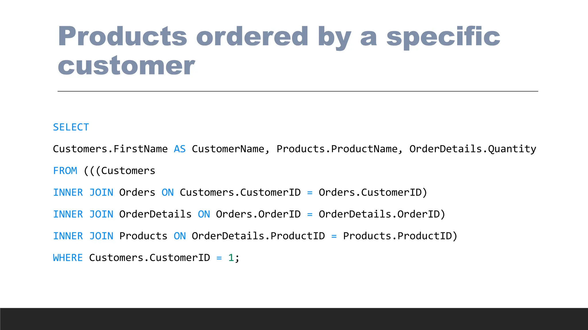
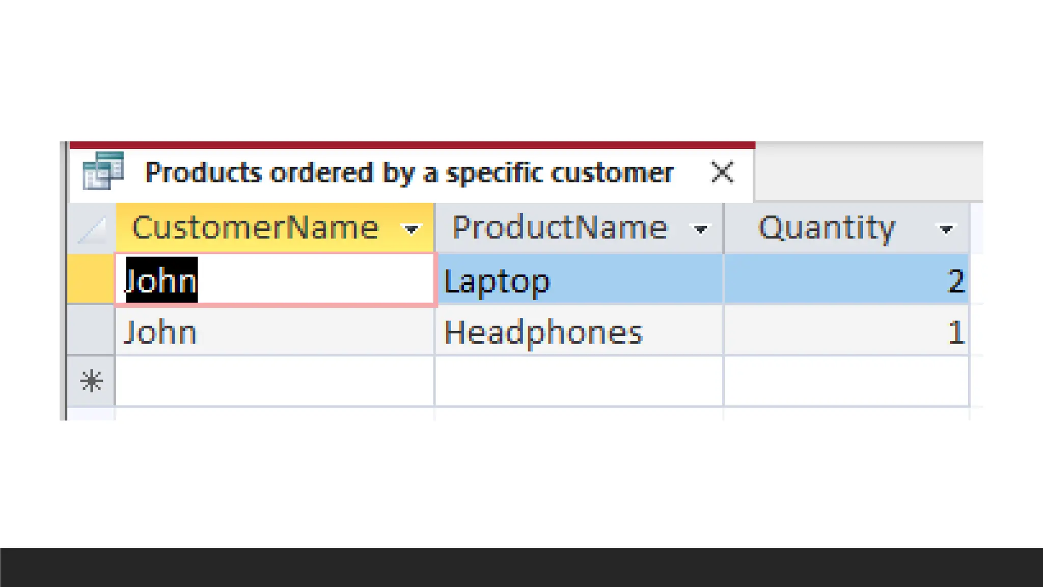
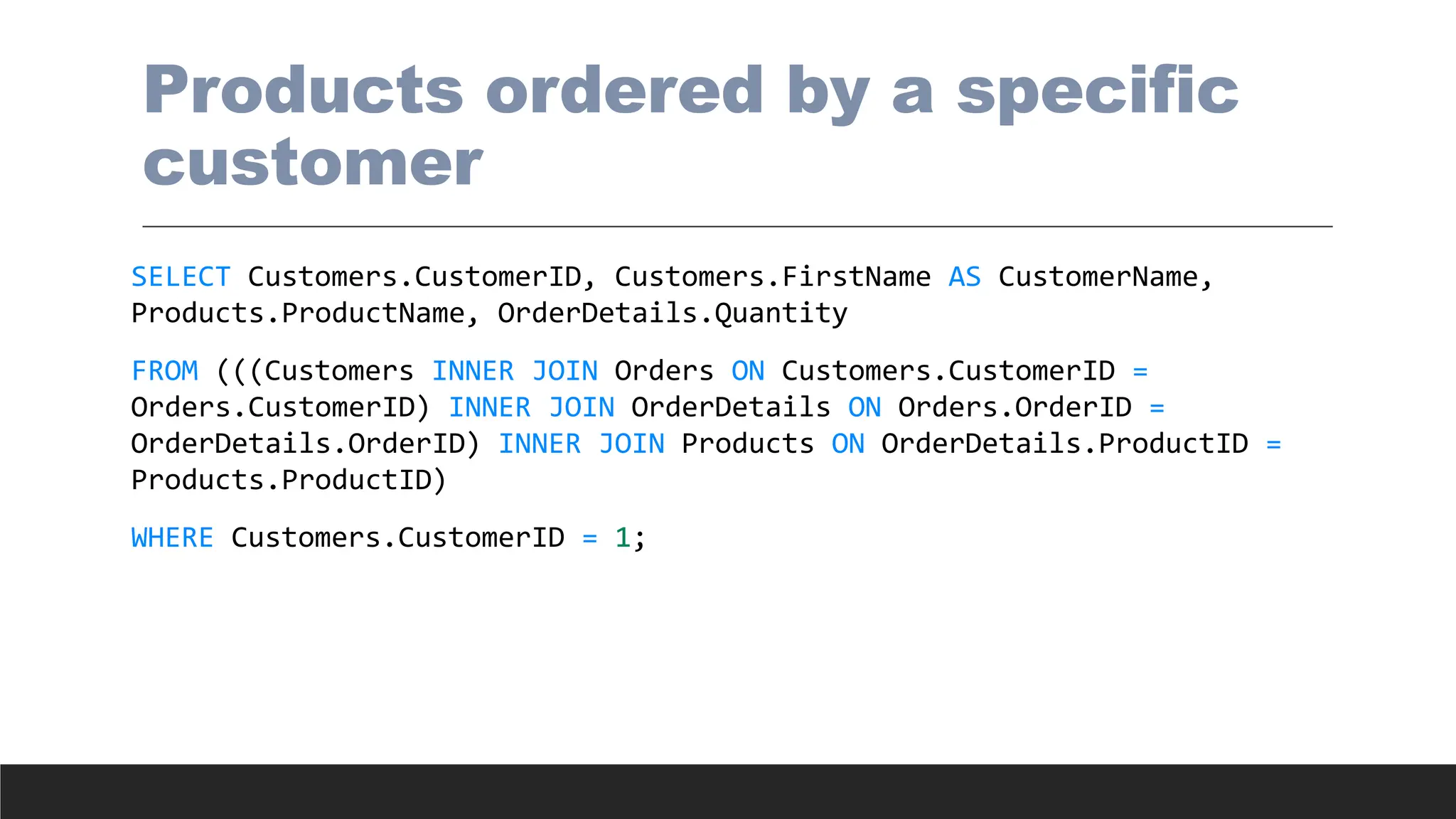
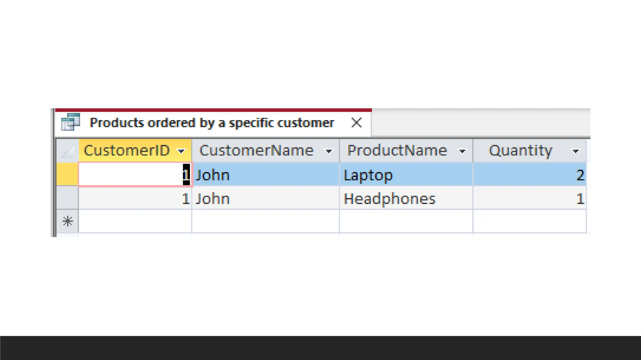
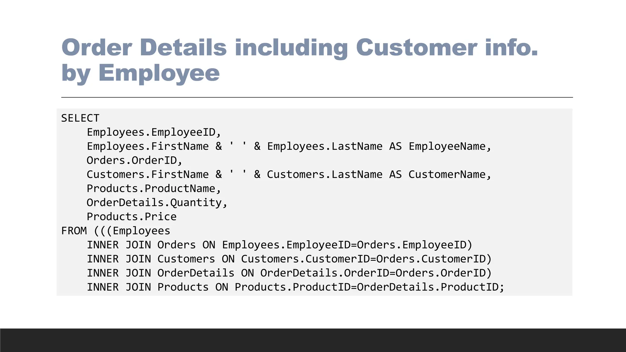
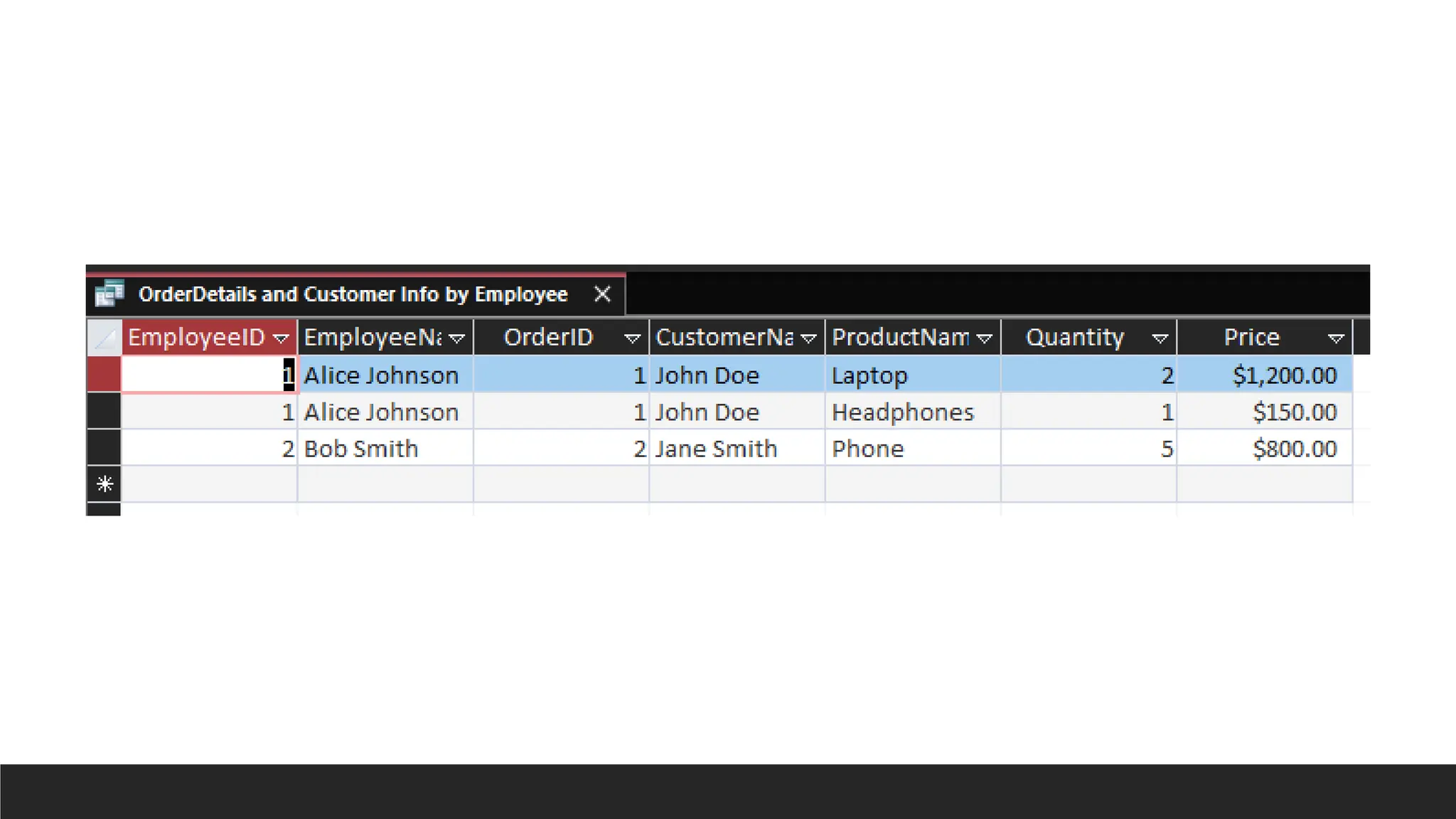

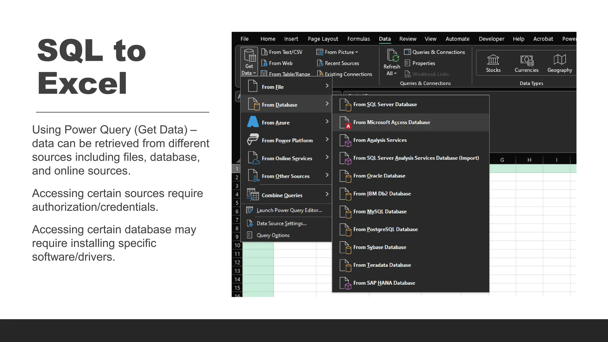
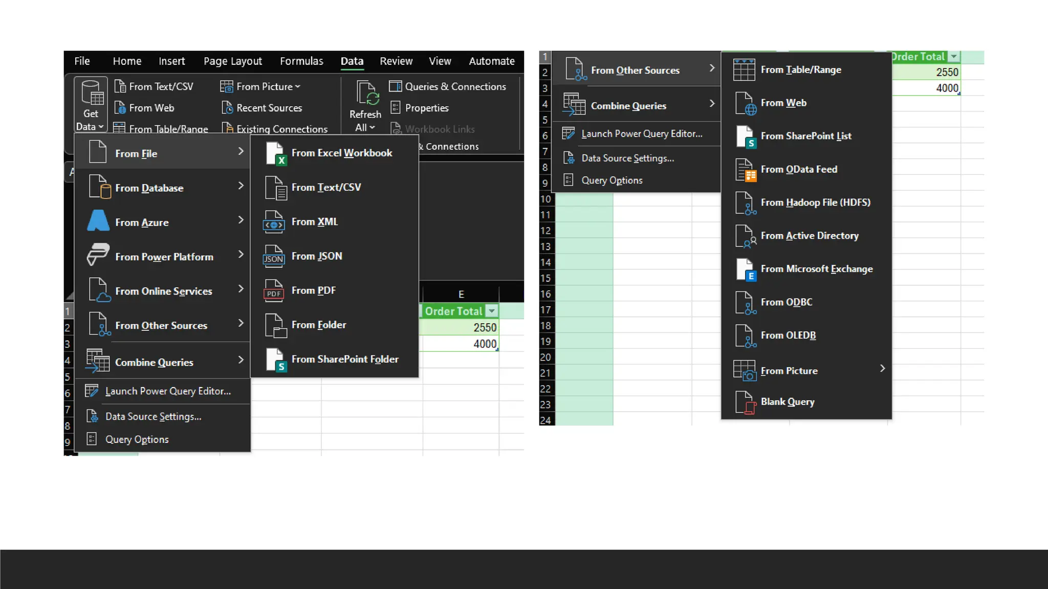
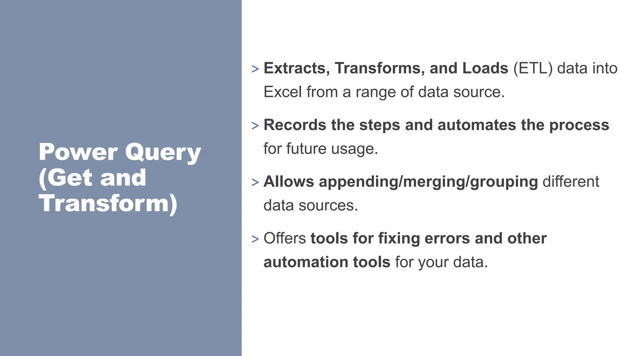
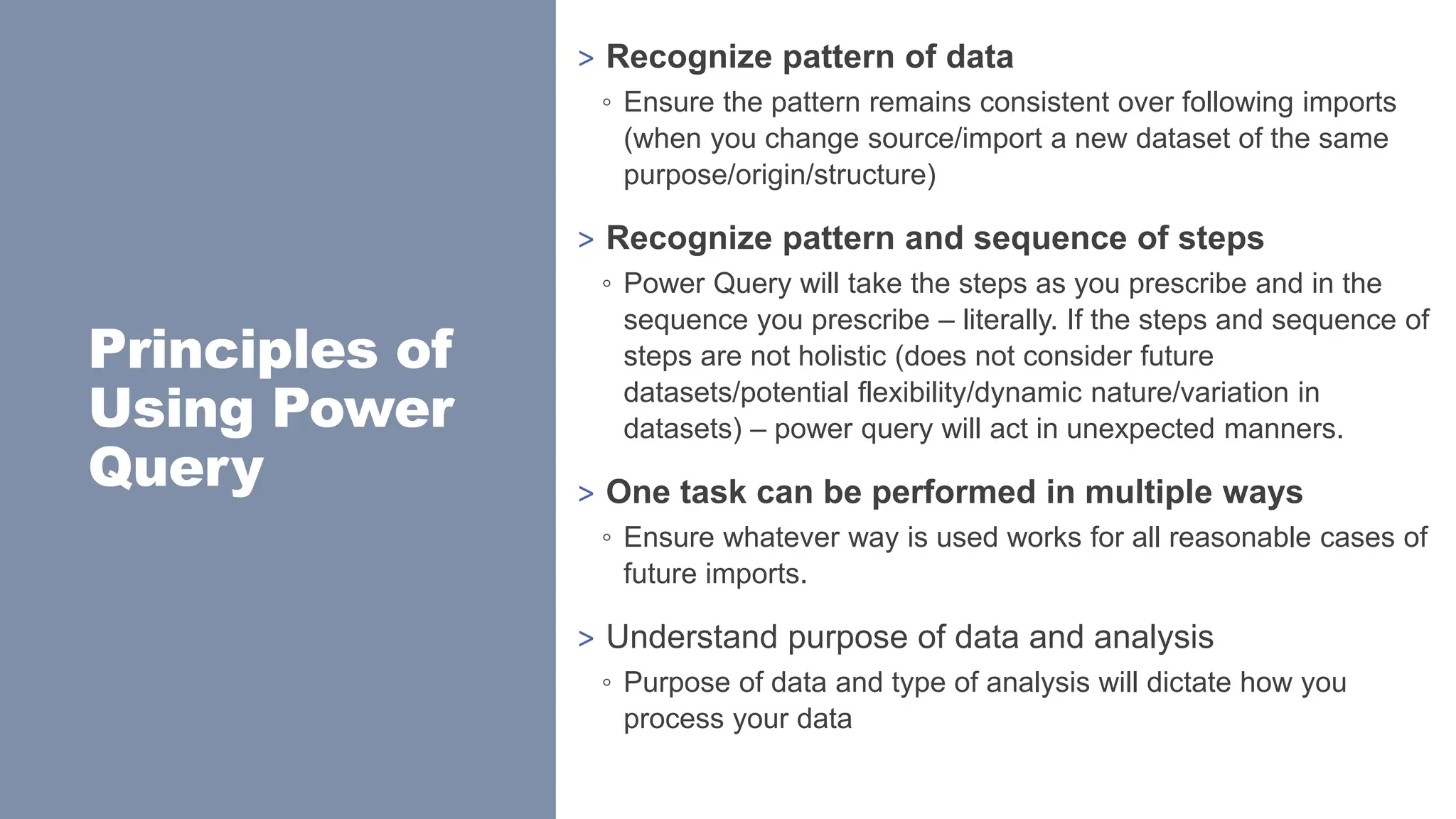
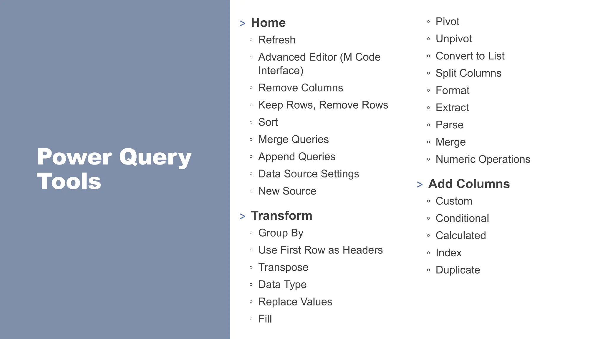
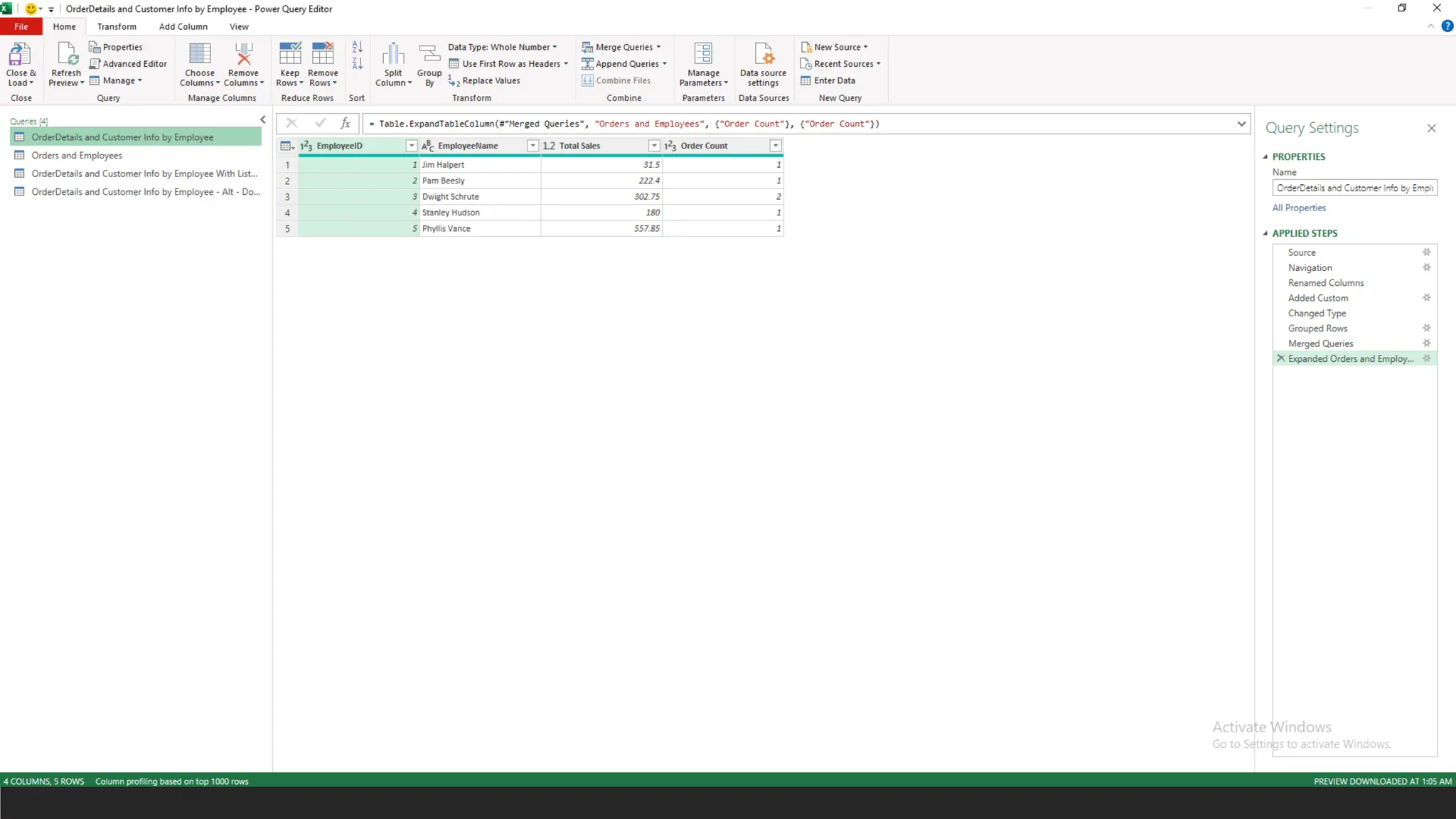
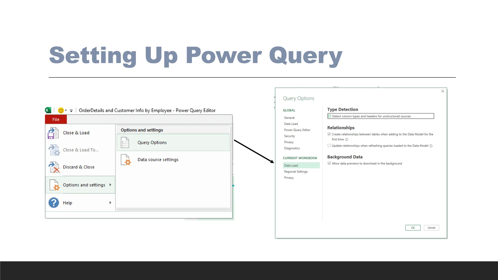
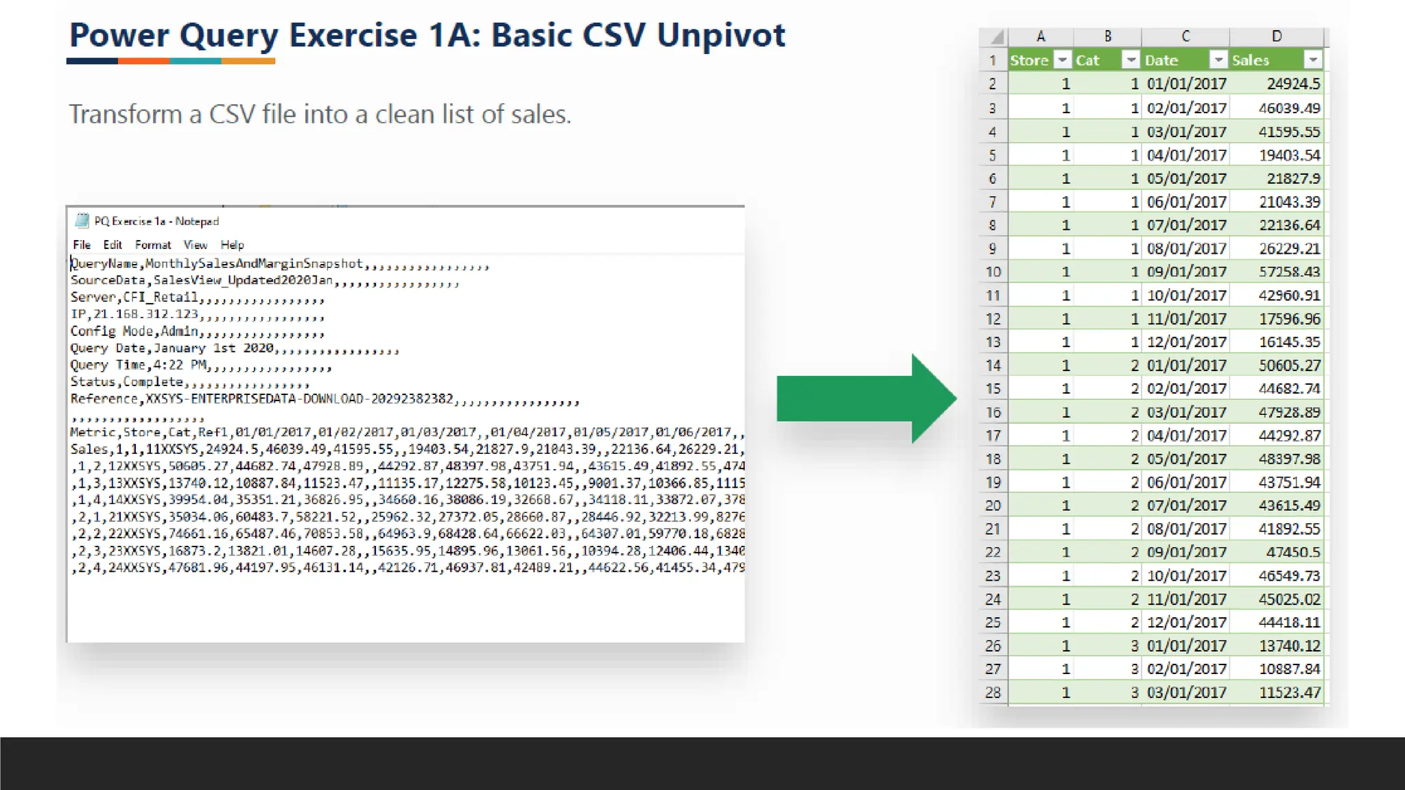
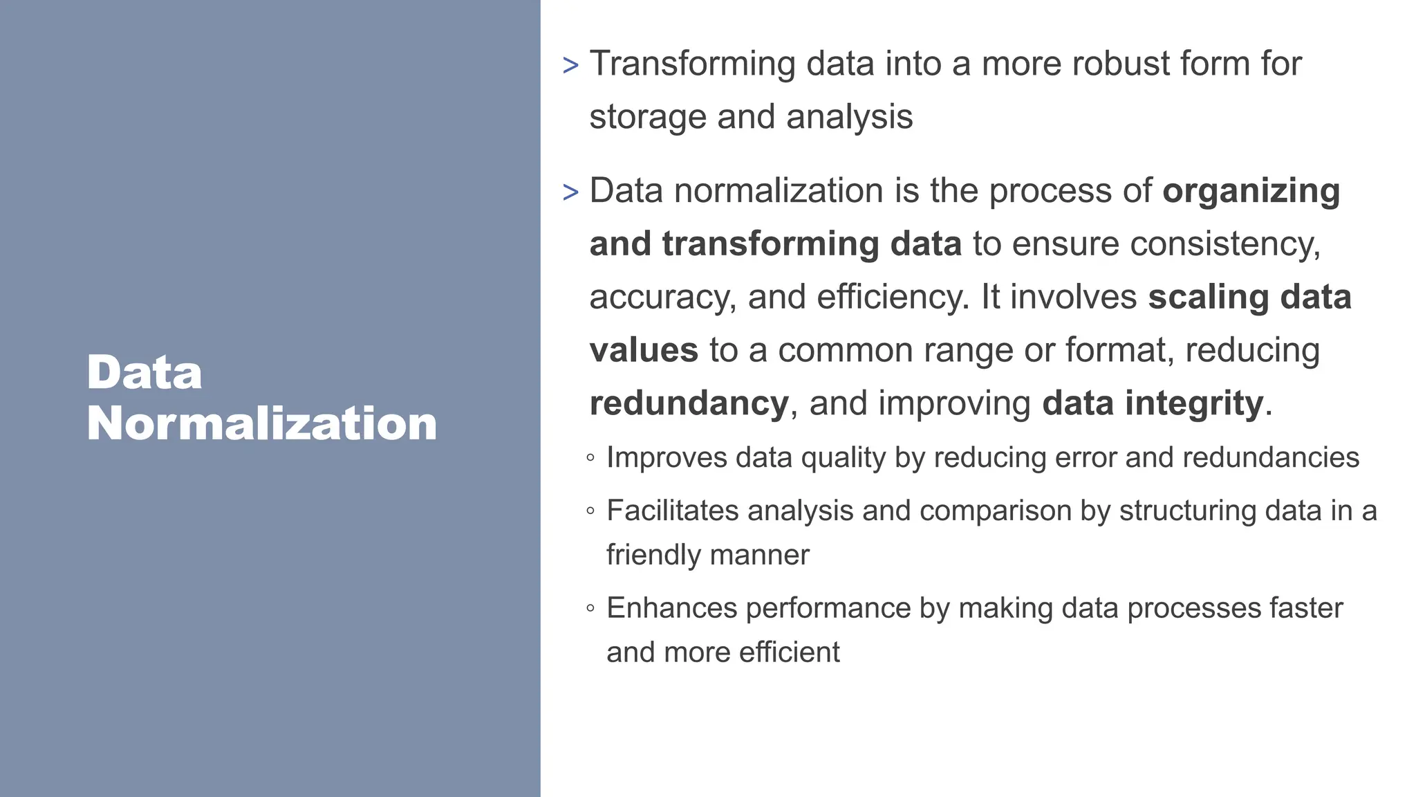
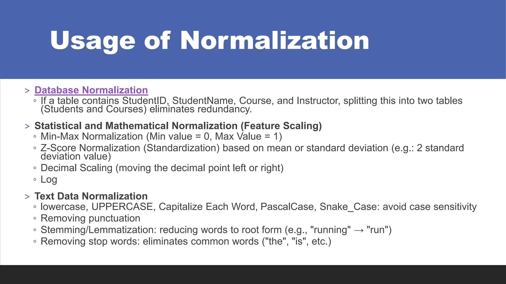
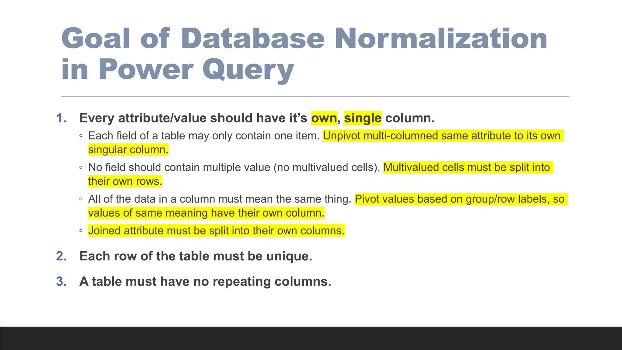
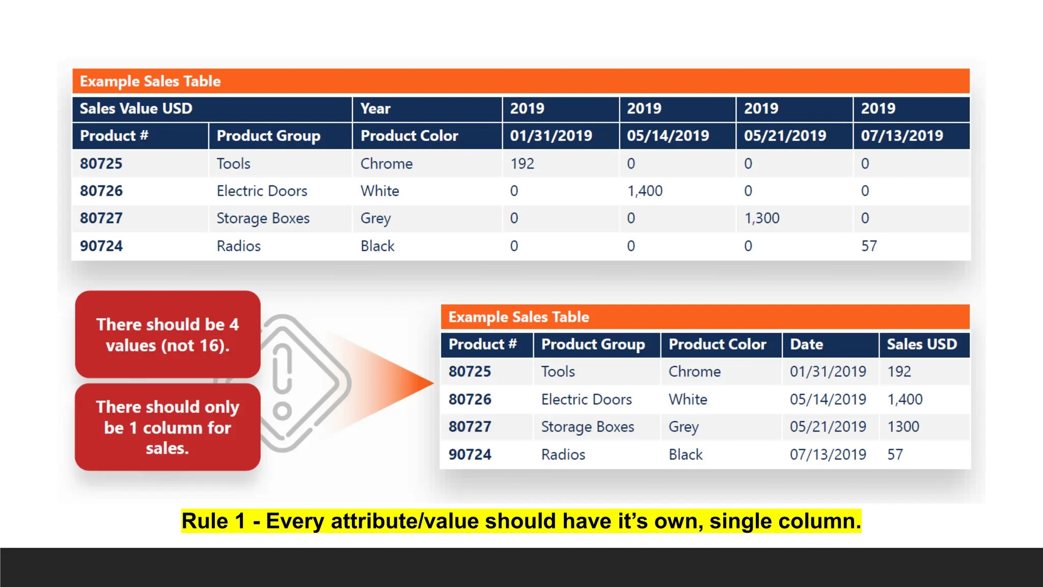
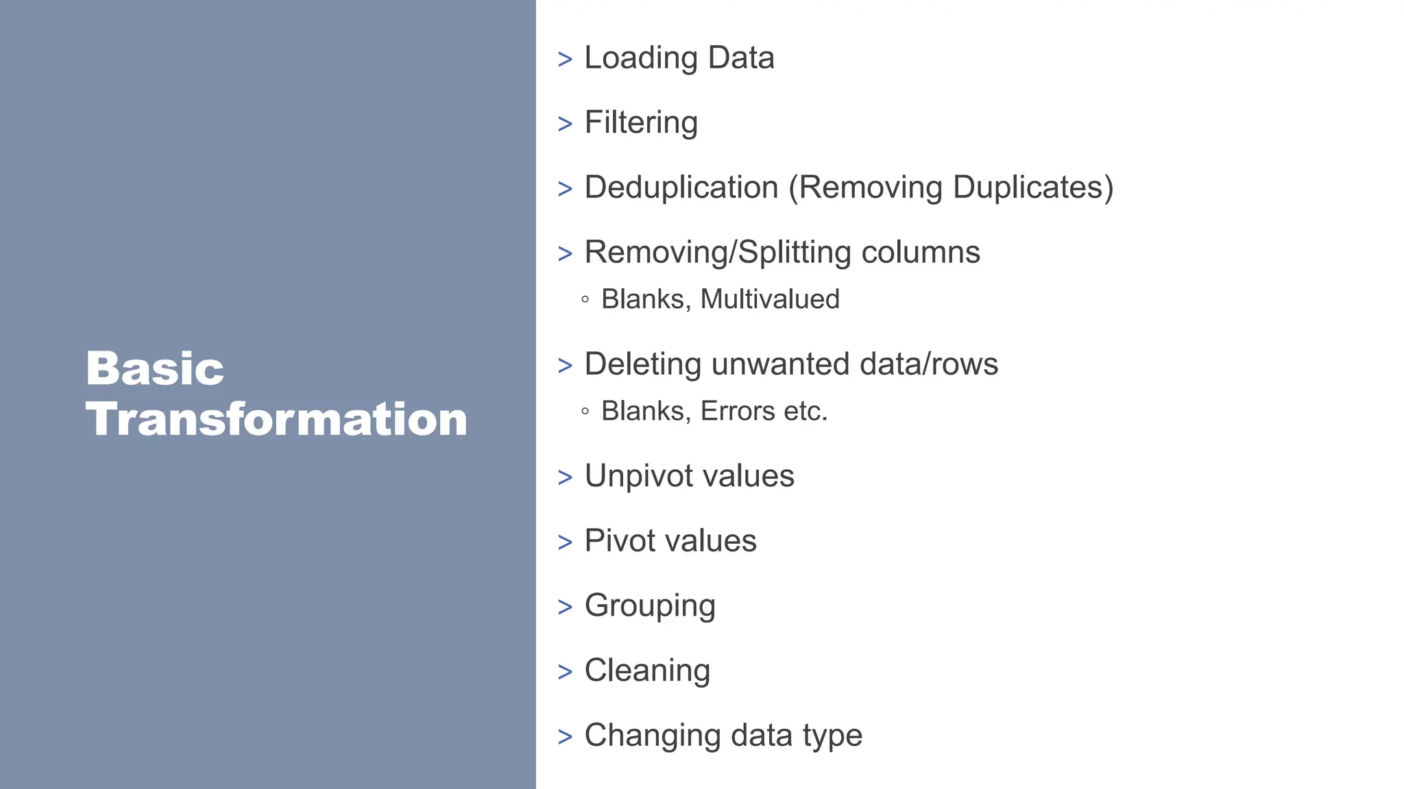
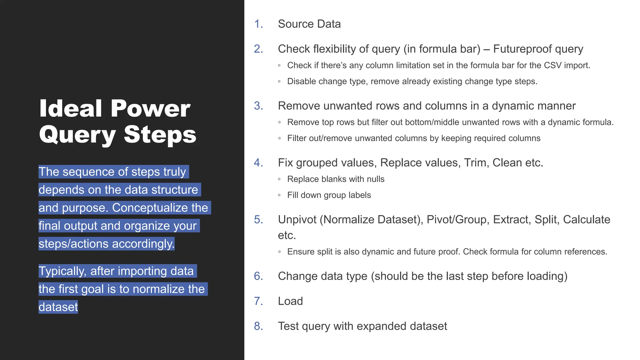
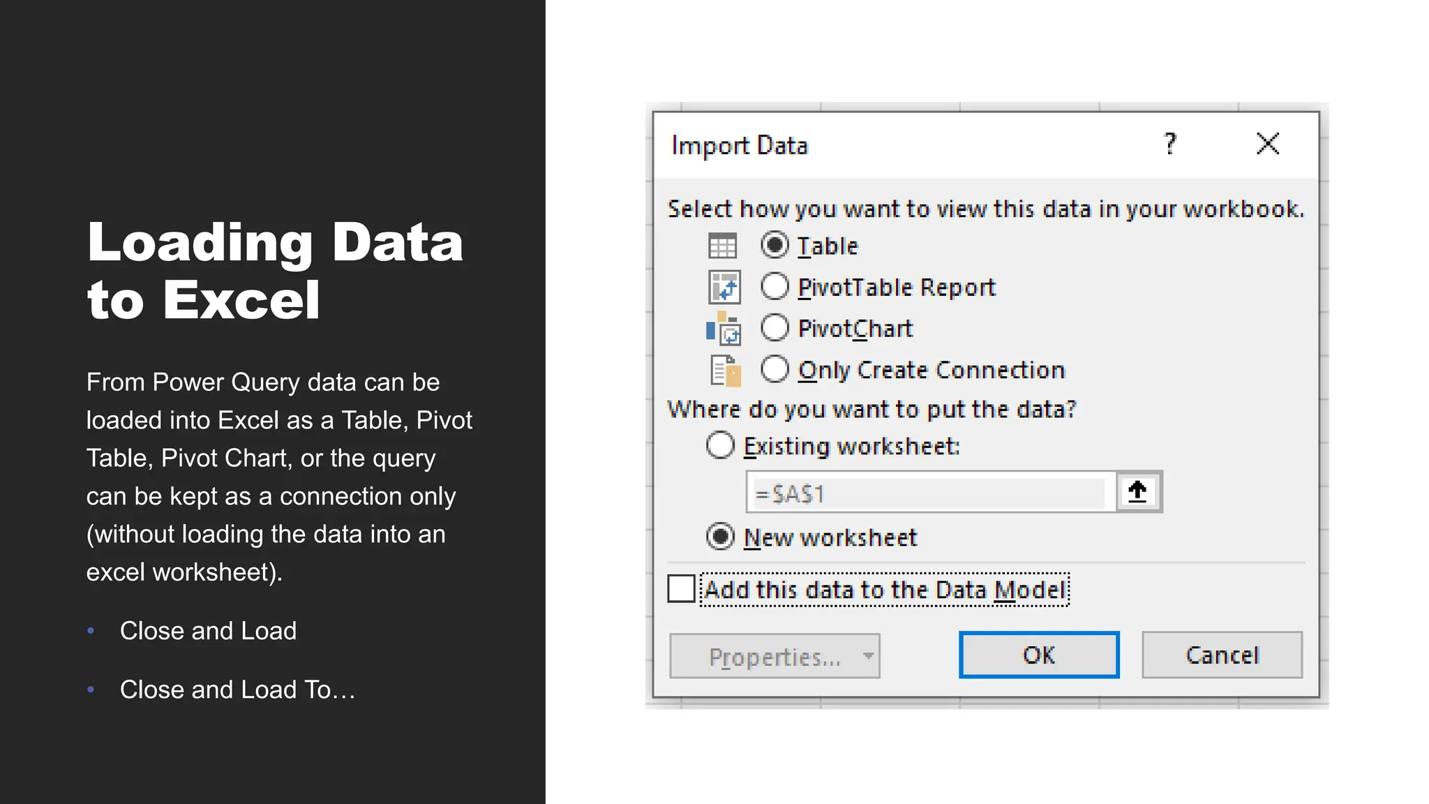
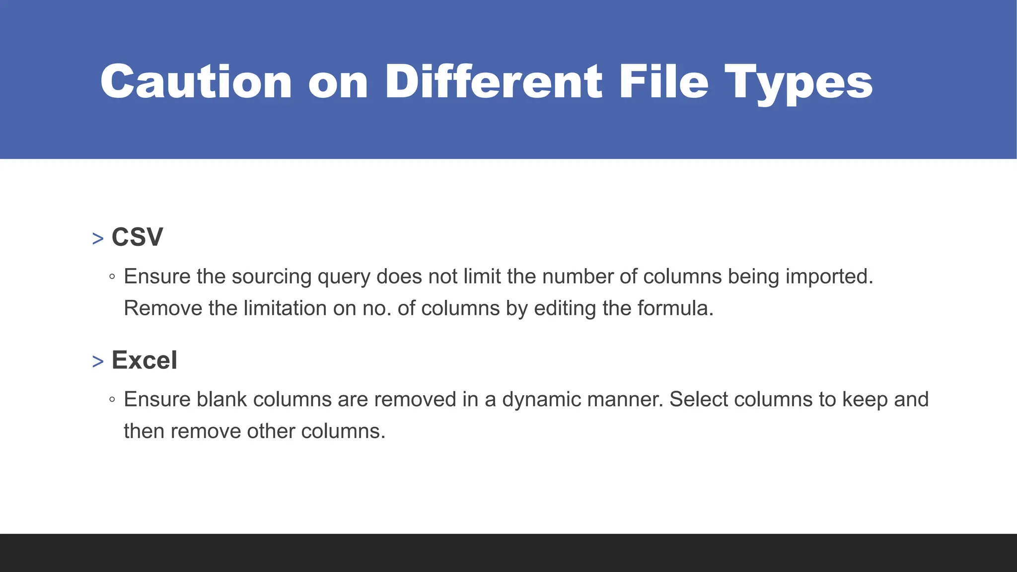
![> = Csv.Document(File.Contents("D:Power Query FundamentalsDataPQ Exercise
1a.csv"),[Delimiter=",", Columns=19, Encoding=1252,
QuoteStyle=QuoteStyle.None])
Remove this to make CSV import dynamic (import as many columns as exists in
subsequent imports/source changes.
= Csv.Document(File.Contents("D:Power Query FundamentalsDataPQ Exercise
1a.csv"),[Delimiter=",", Encoding=1252, QuoteStyle=QuoteStyle.None])](https://image.slidesharecdn.com/2-250703033149-22abe271/75/Data-Retrieval-and-Preparation-Business-Analytics-pdf-179-2048.jpg)
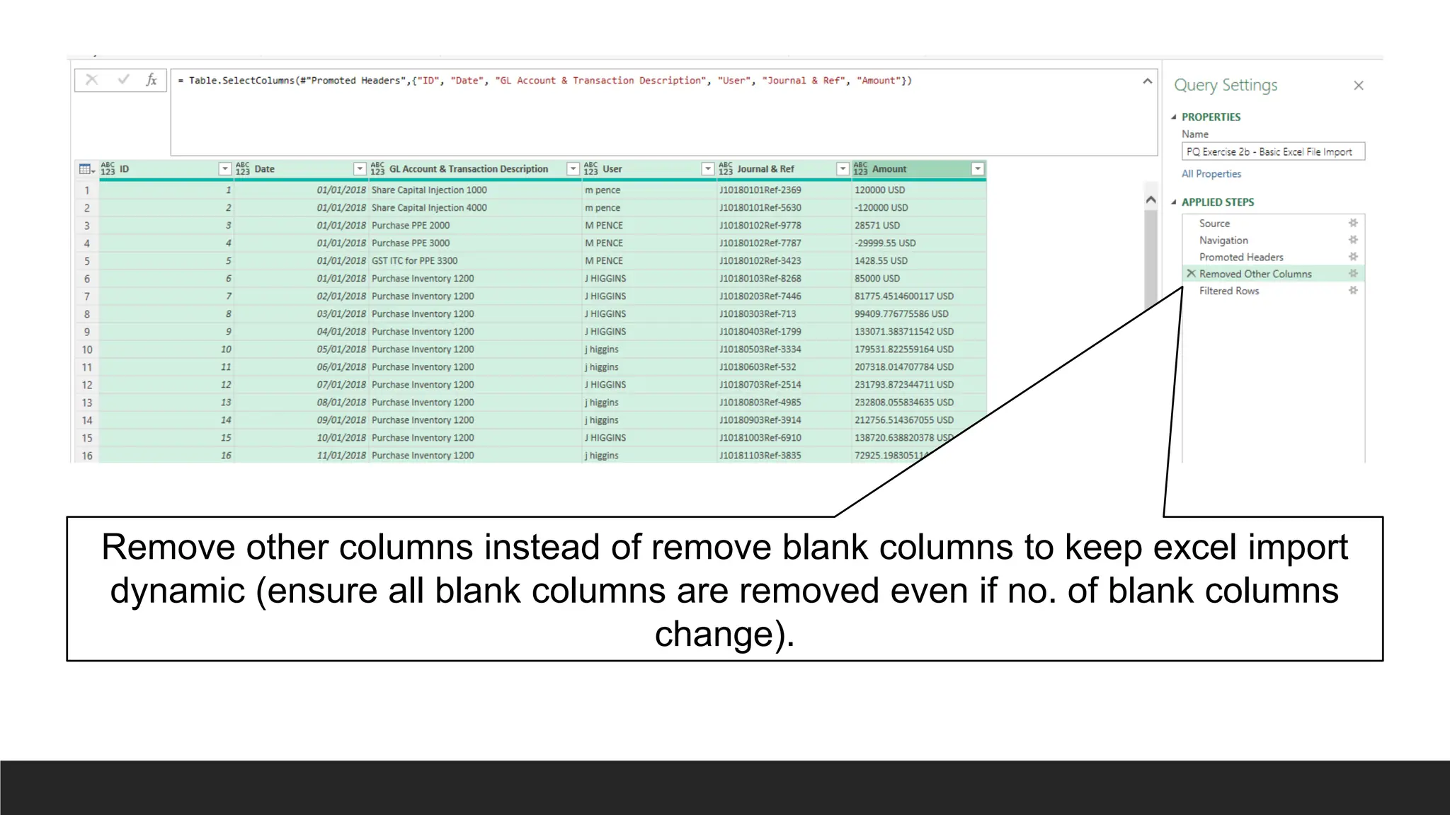

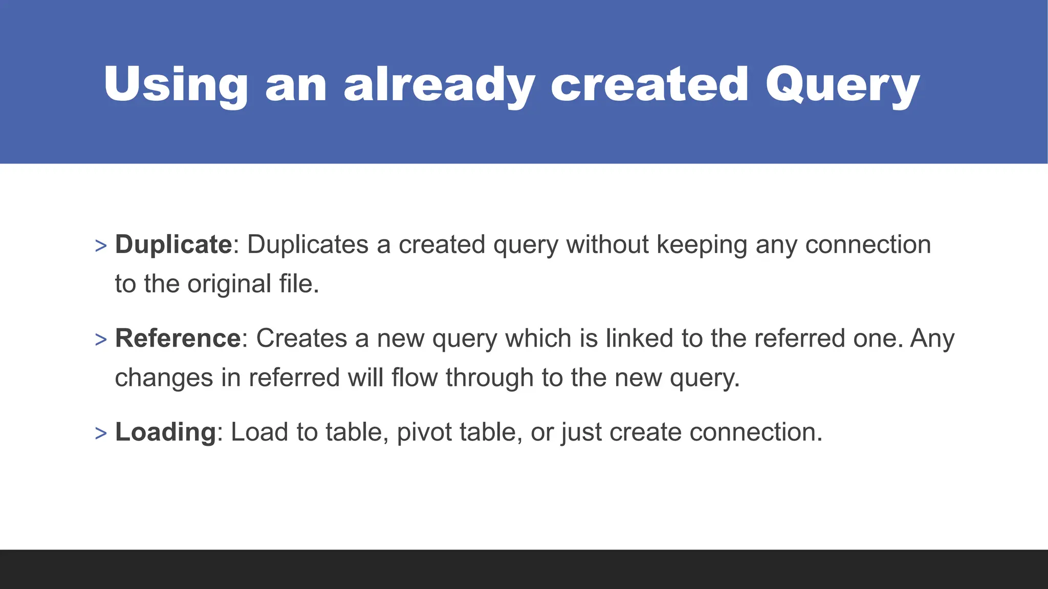
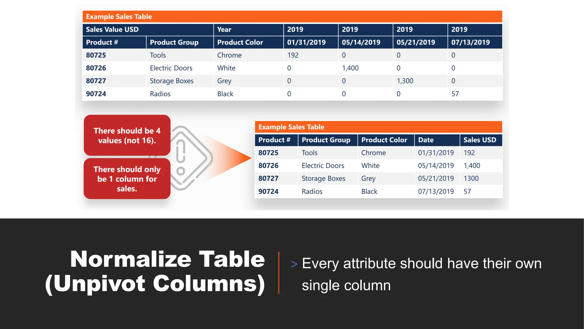
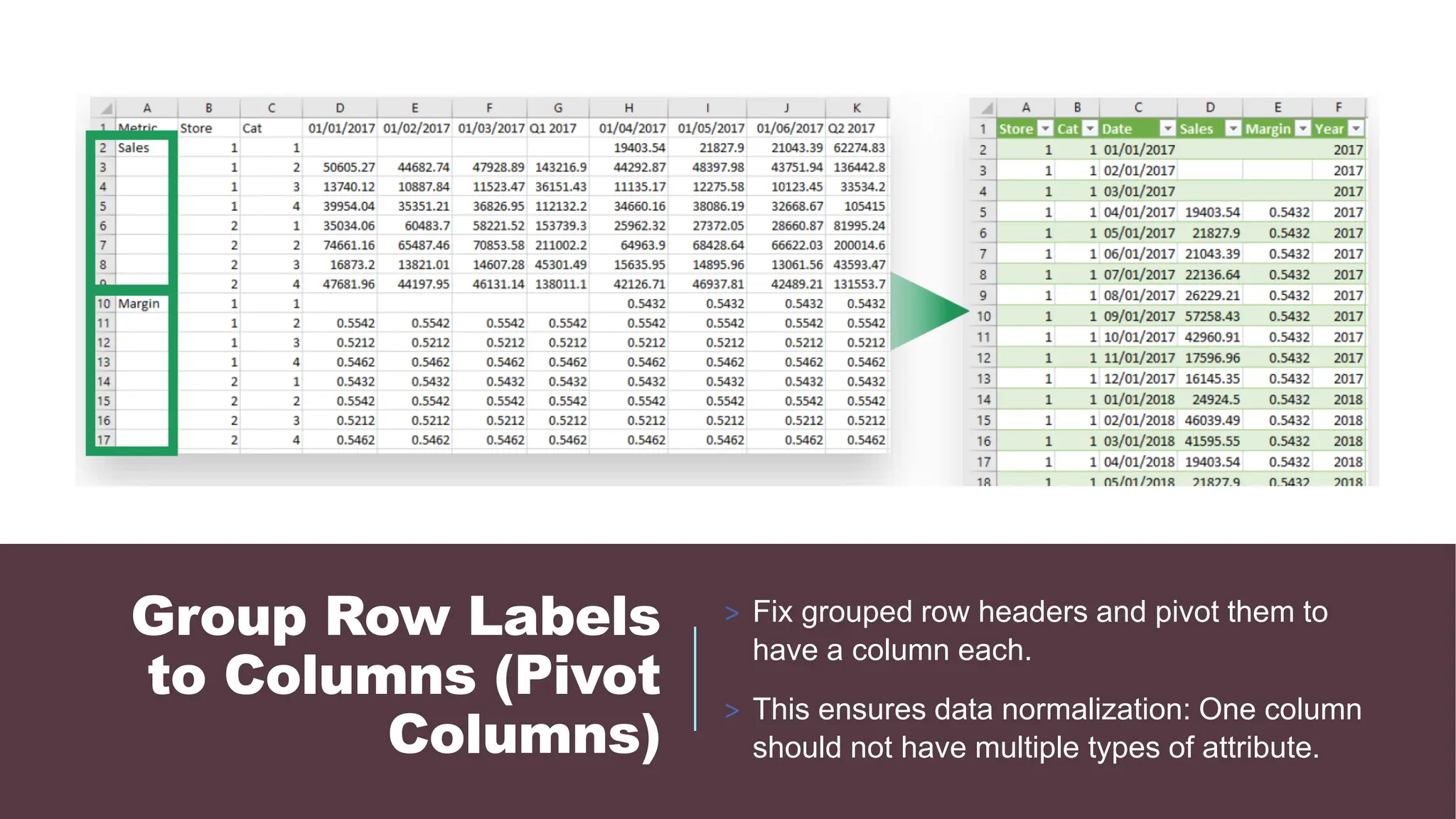
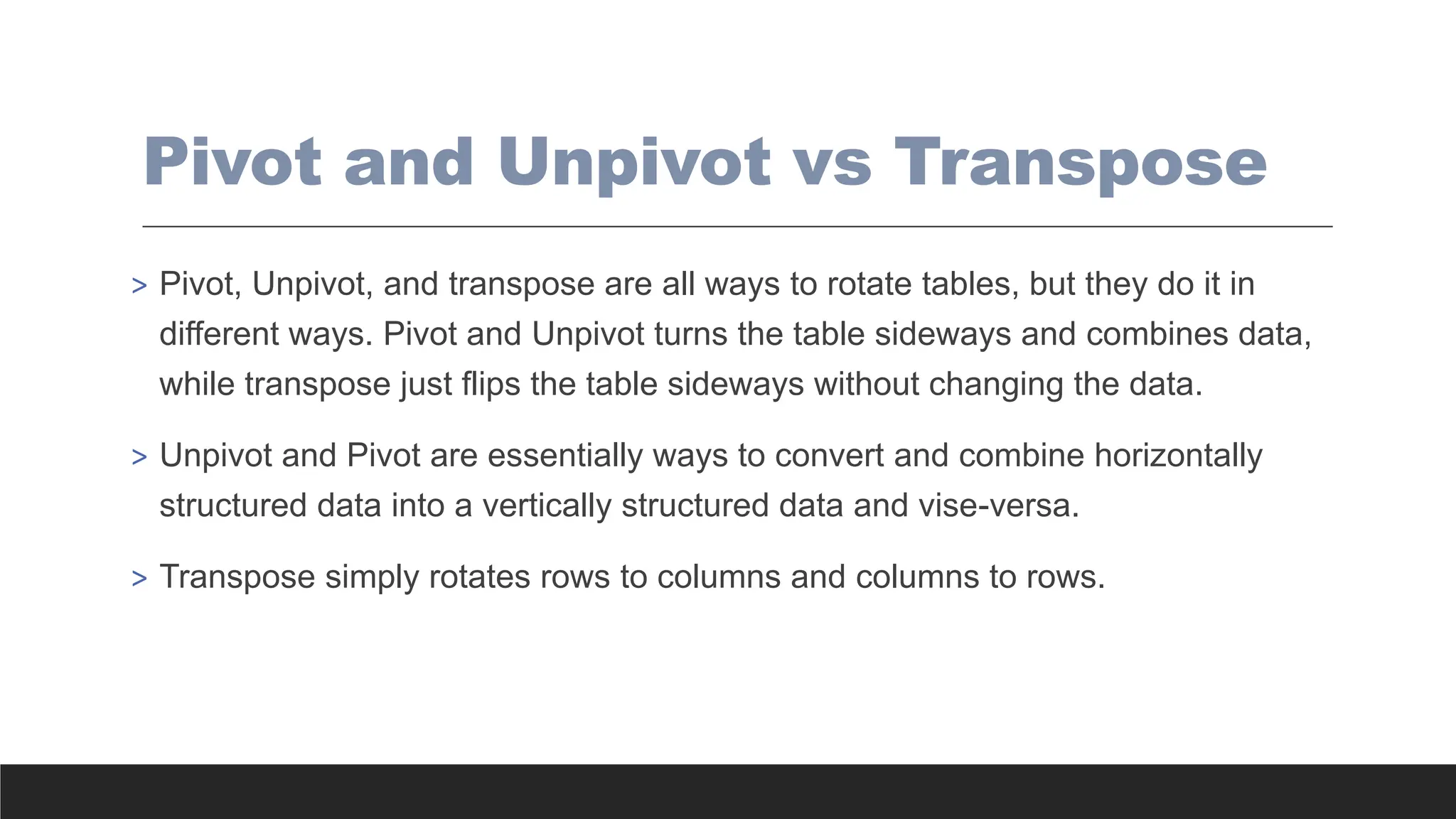
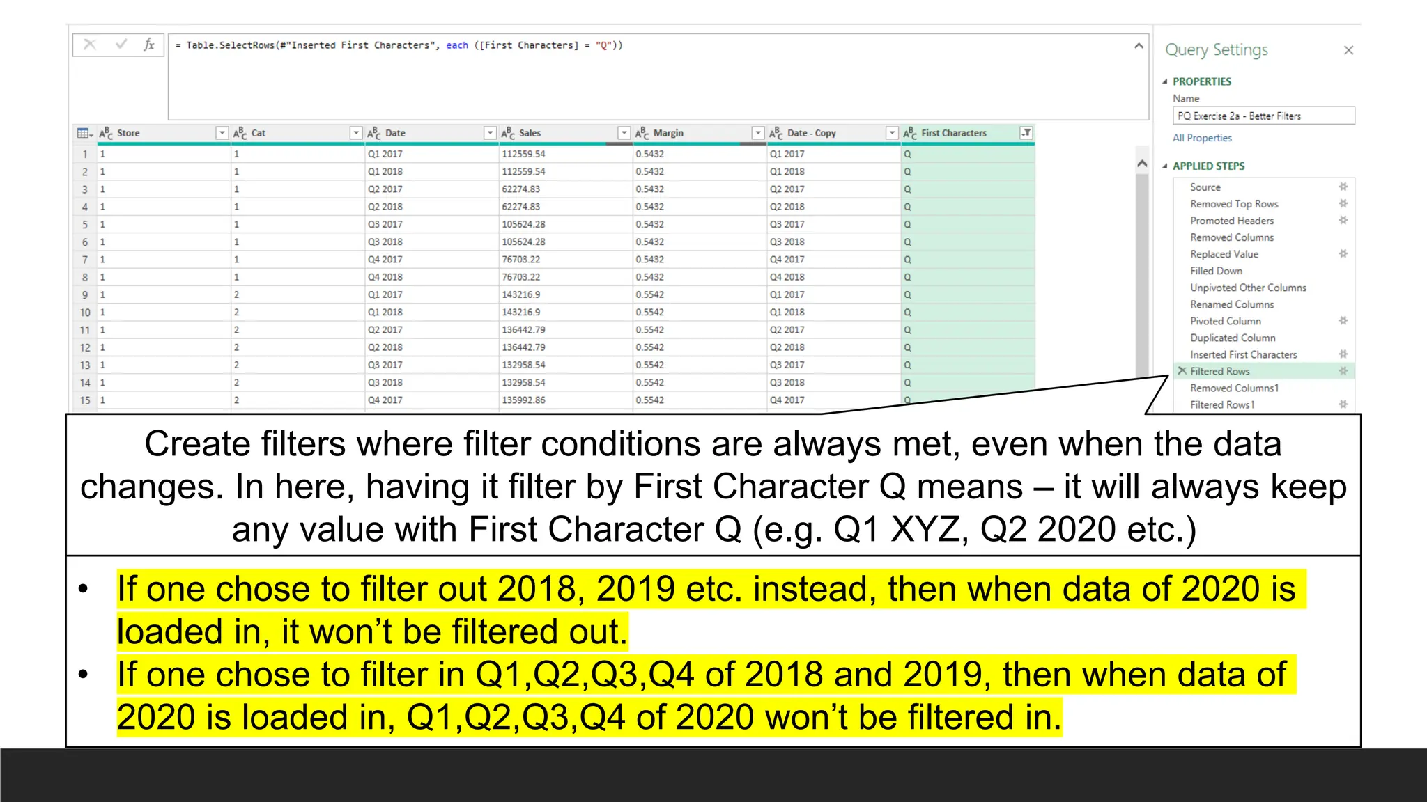
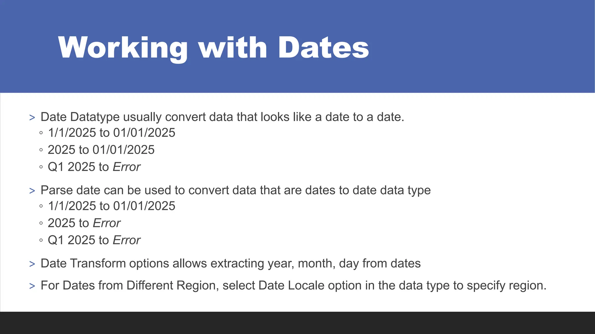
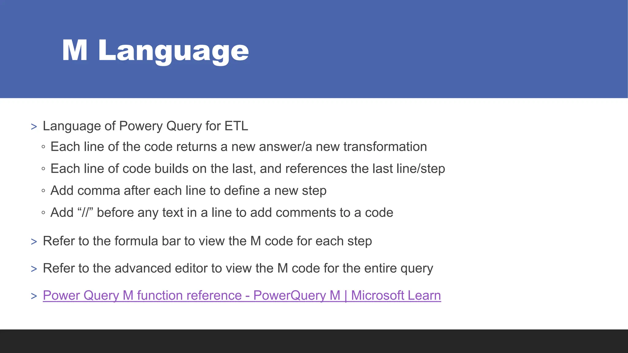
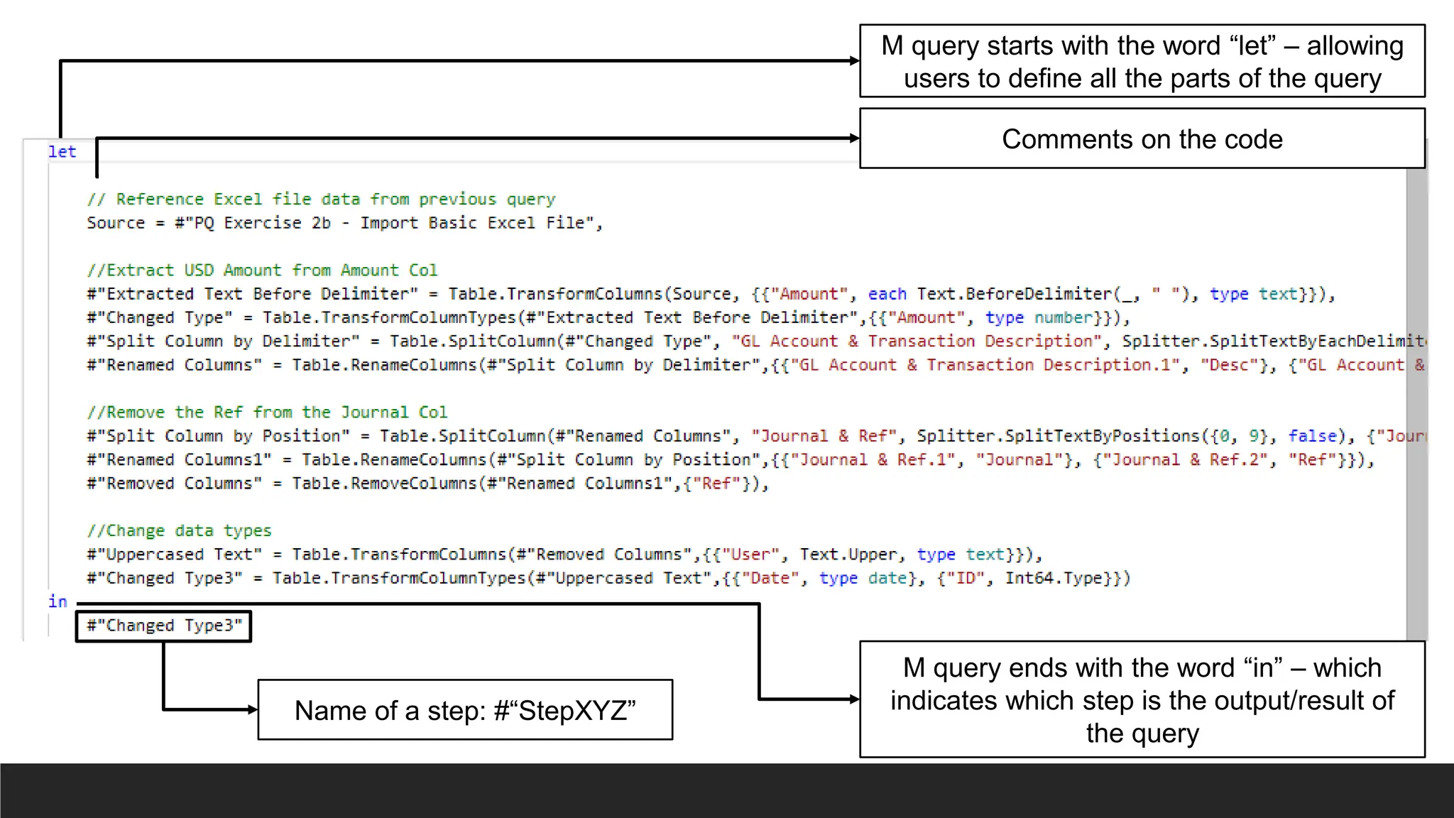
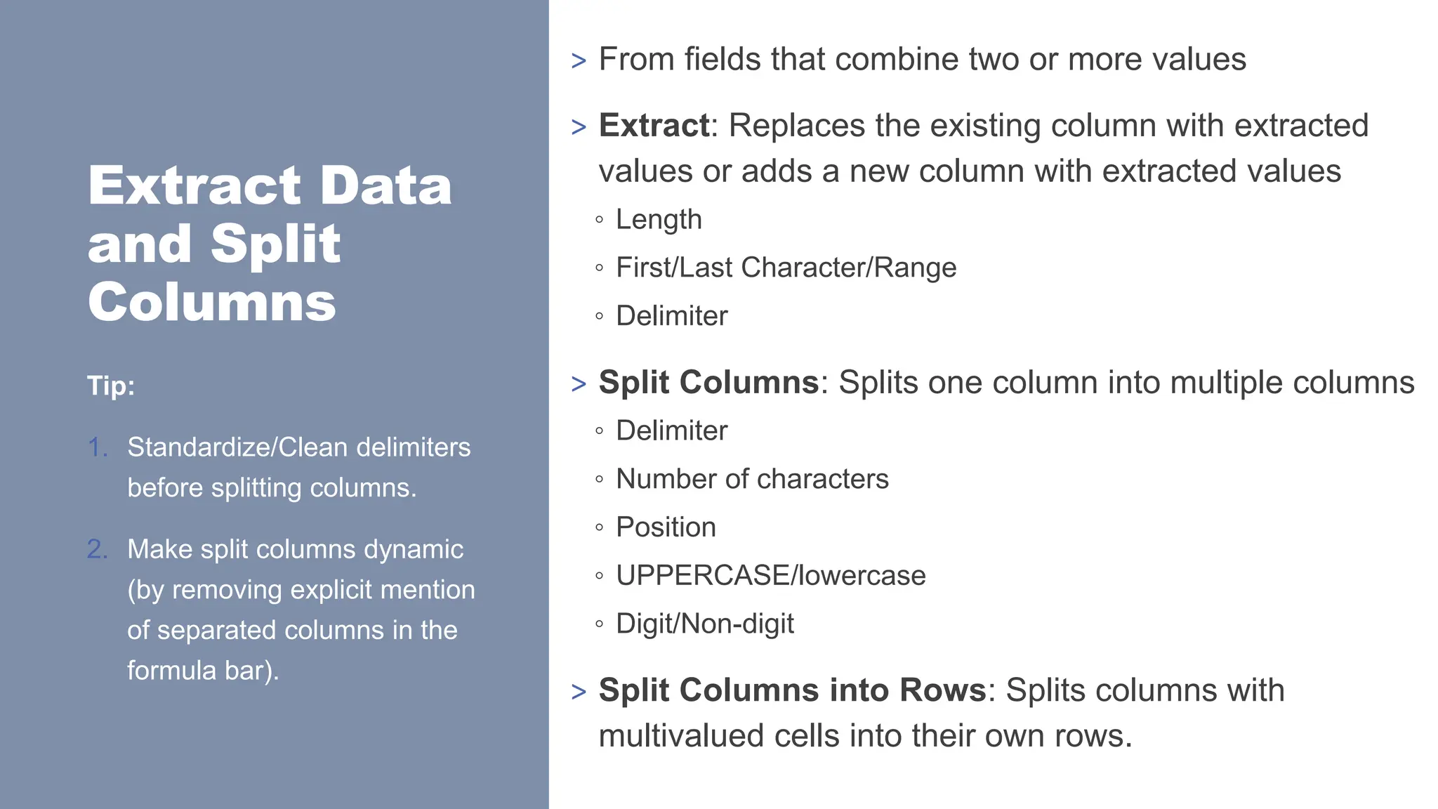
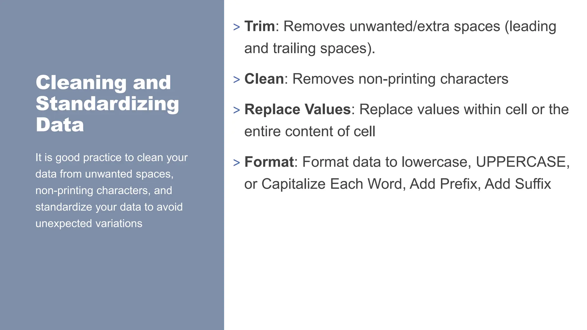
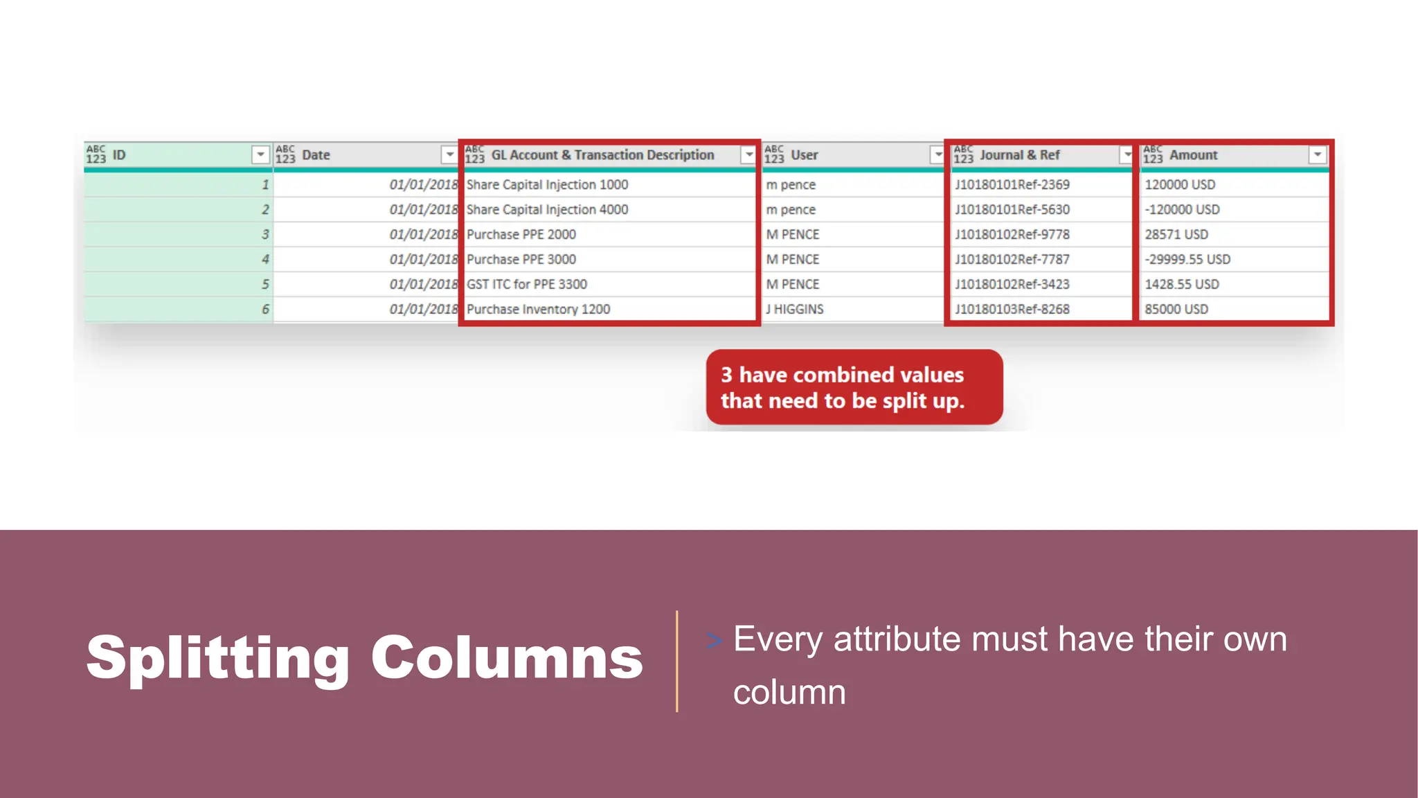
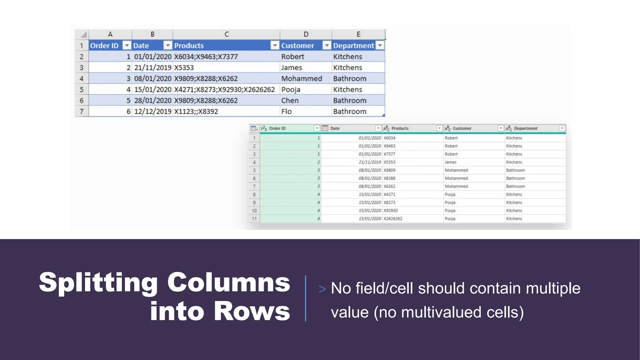
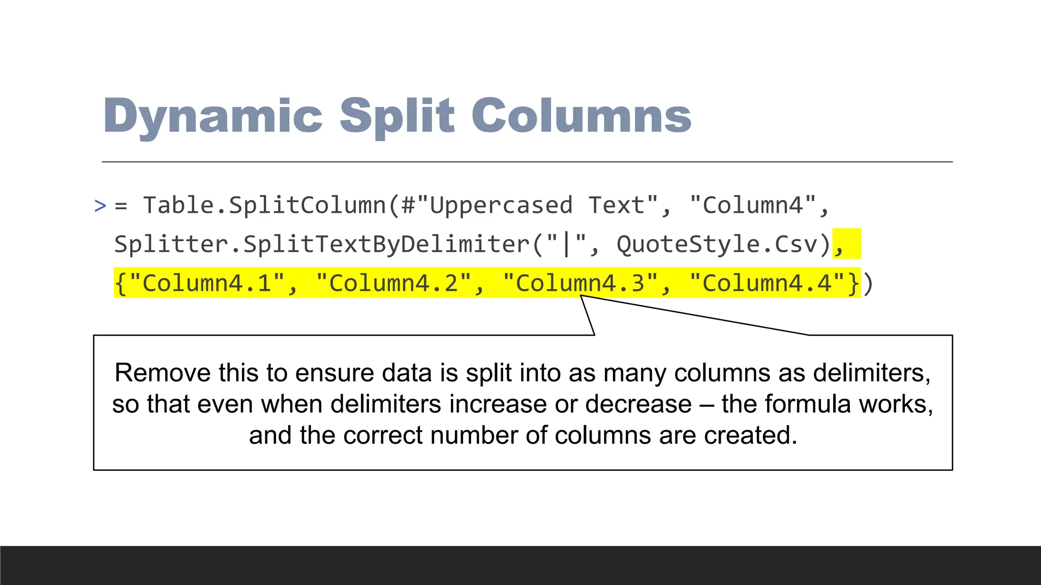
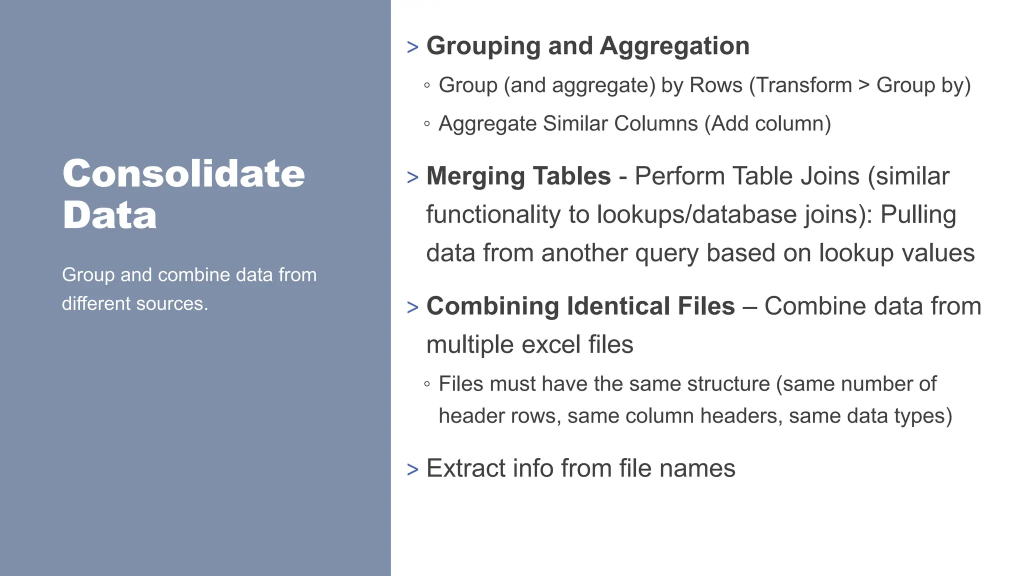
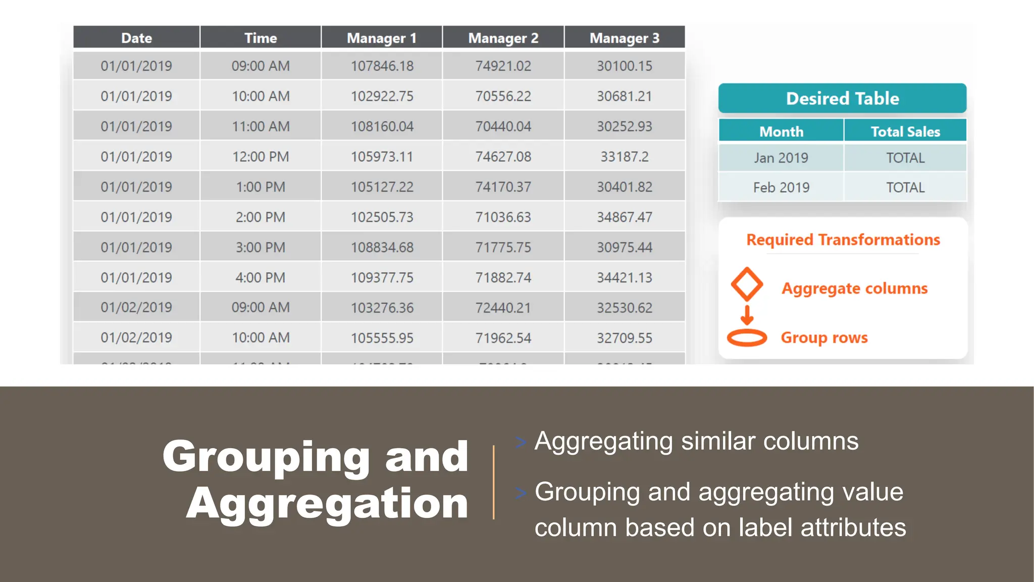
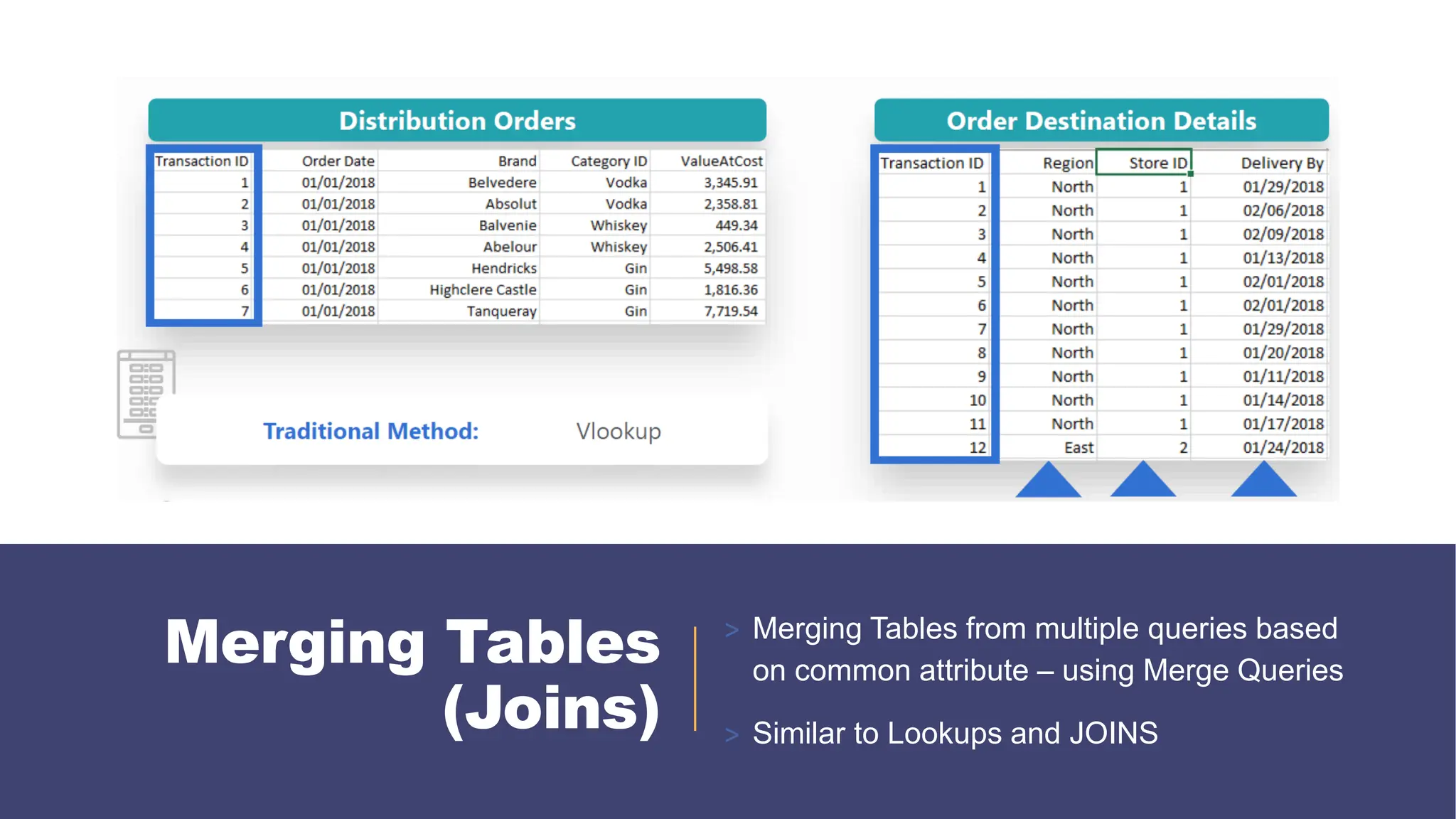
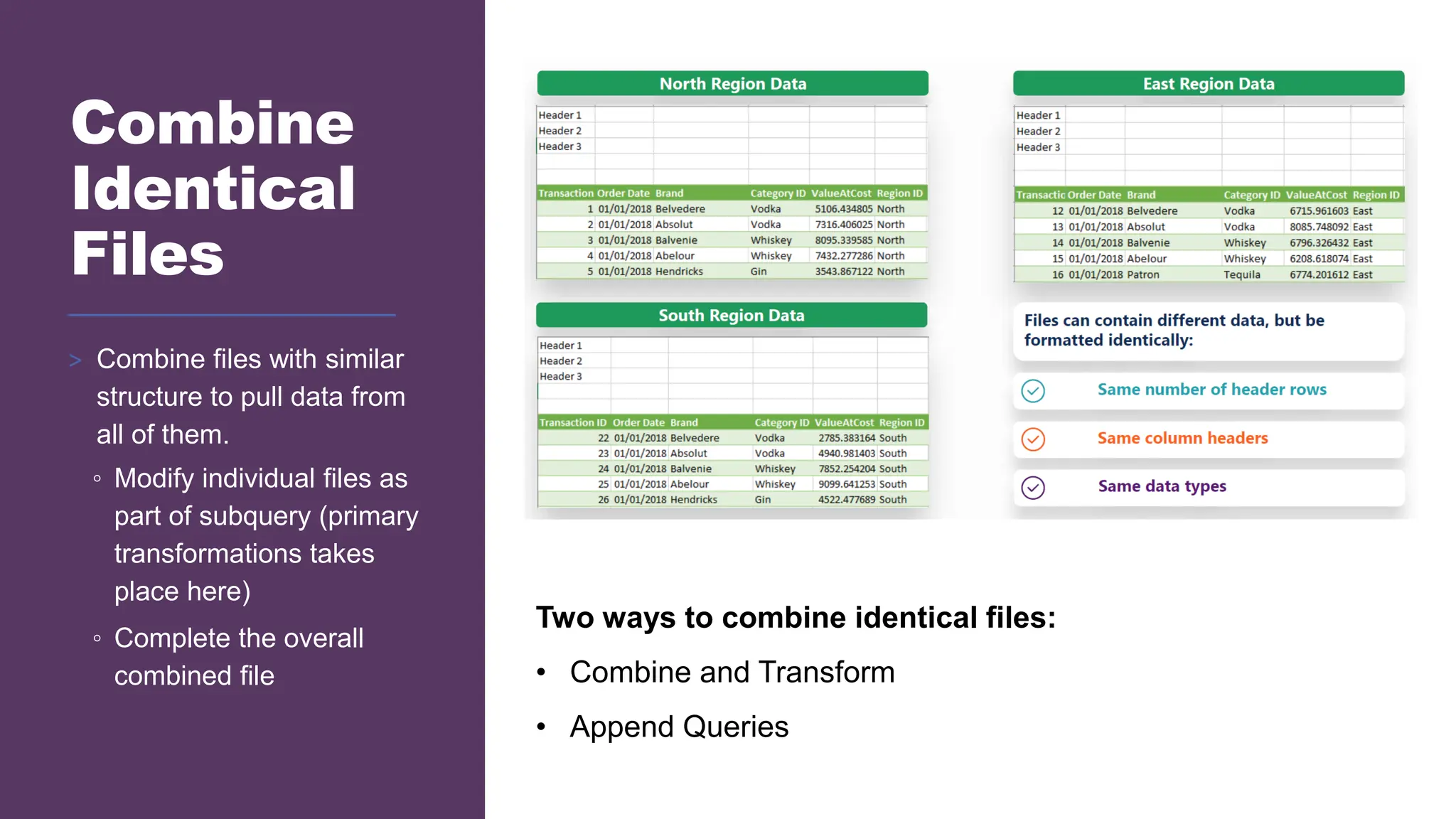
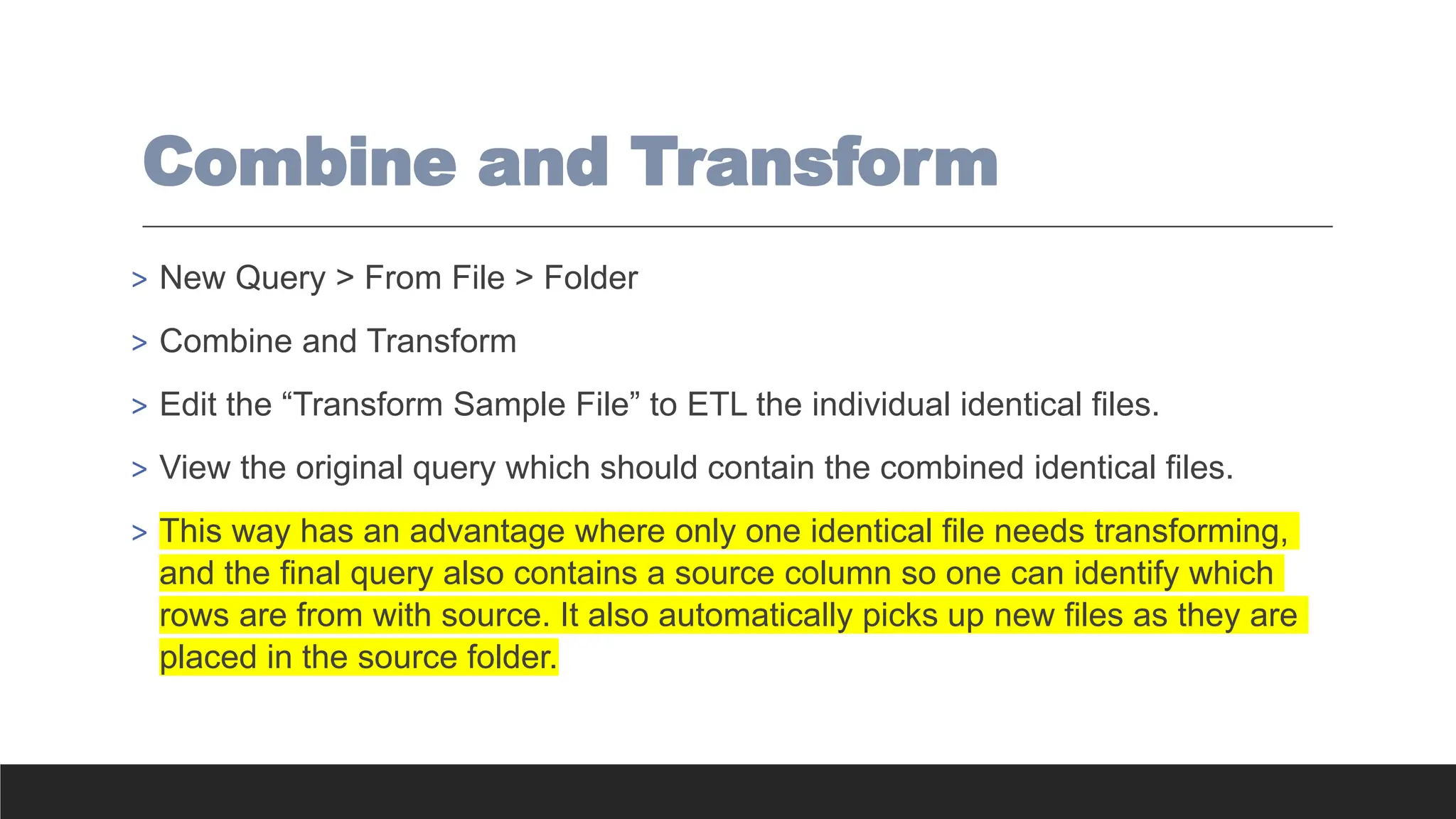
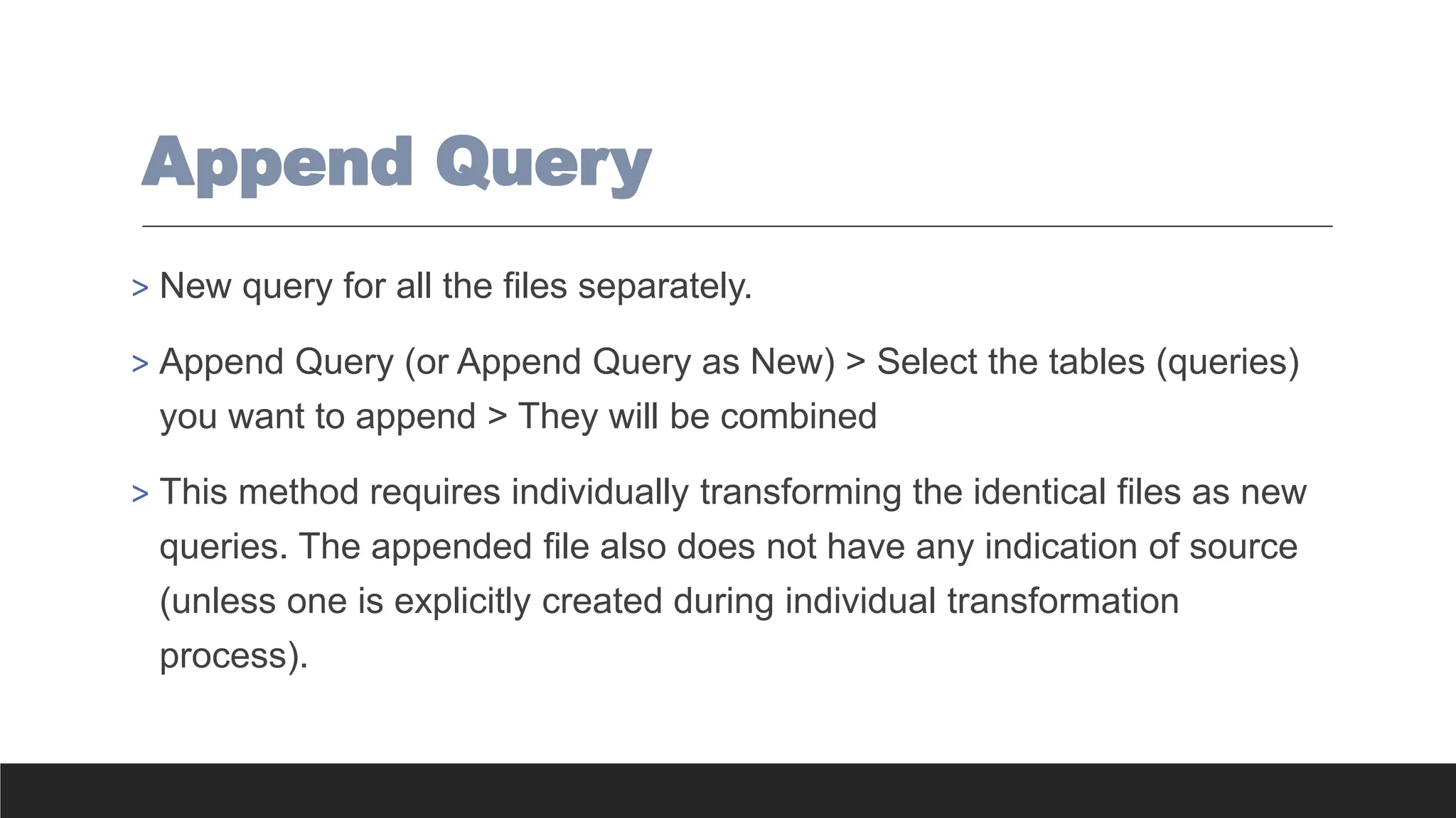
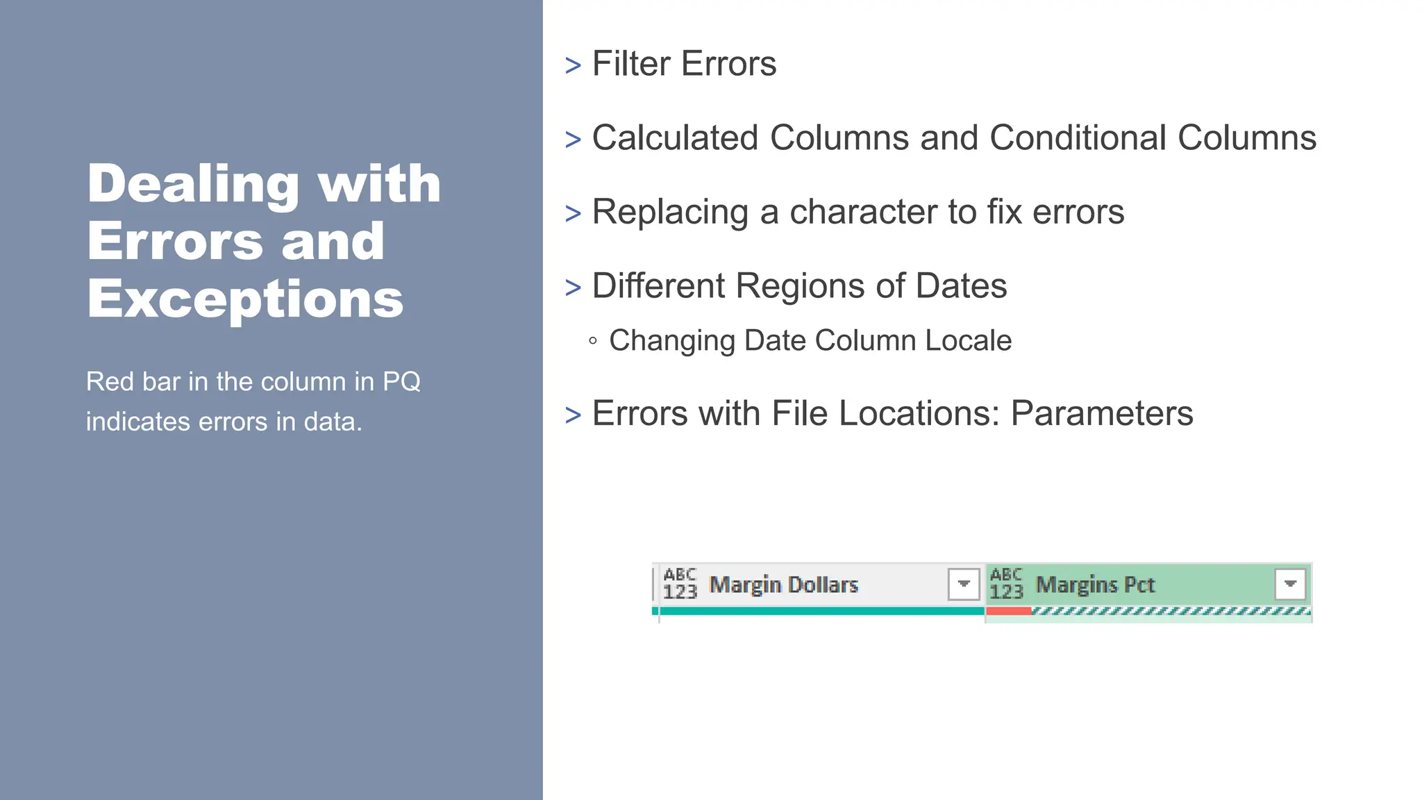
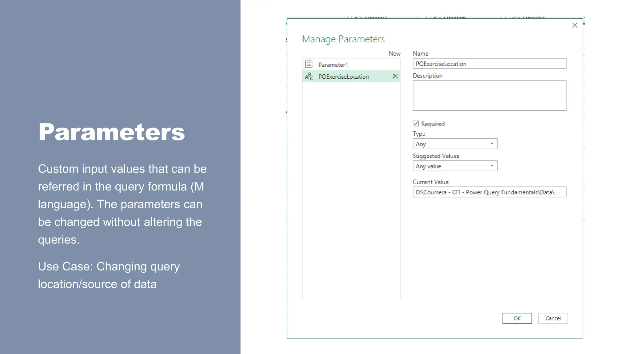
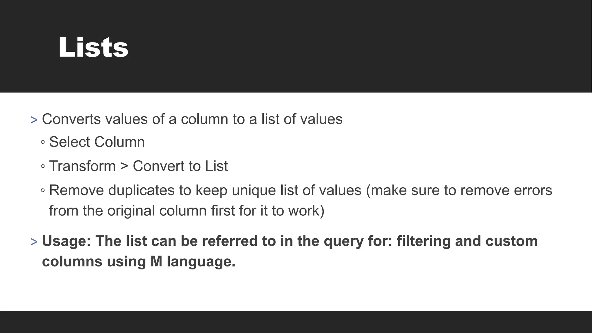
![Lookup with Custom Columns
> =Table[ColumnToReturn]{List.PositionOf(Table[ColumnToMatch],[ColumnToLook
Up])}
> =Categories[Category]{List.PositionOf(Categories[Acronym],[Cat])}
> This finds the position of [Cat] in Categories[Acronym], then returns
Categories[Category] from the same position. Similar to a Lookup.
> = Table.AddColumn(#“LastStep", "Category", each
Categories[Category]{List.PositionOf(Categories[Acronym],[Cat])})](https://image.slidesharecdn.com/2-250703033149-22abe271/75/Data-Retrieval-and-Preparation-Business-Analytics-pdf-205-2048.jpg)
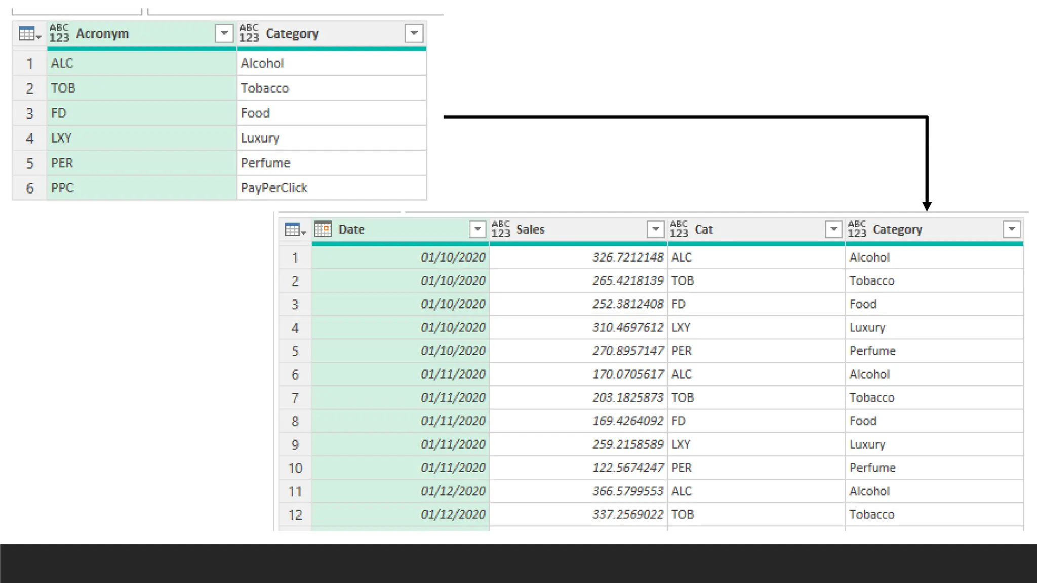
![Count Distinct Values for Each
Group with M
= Table.Group(#"Changed Type", {"EmployeeID", "EmployeeName"}, {{"Total Sales",
each List.Sum([Total]), type nullable number},{"Number of Orders", each
List.Count(List.Distinct([OrderID])), type number}})](https://image.slidesharecdn.com/2-250703033149-22abe271/75/Data-Retrieval-and-Preparation-Business-Analytics-pdf-207-2048.jpg)

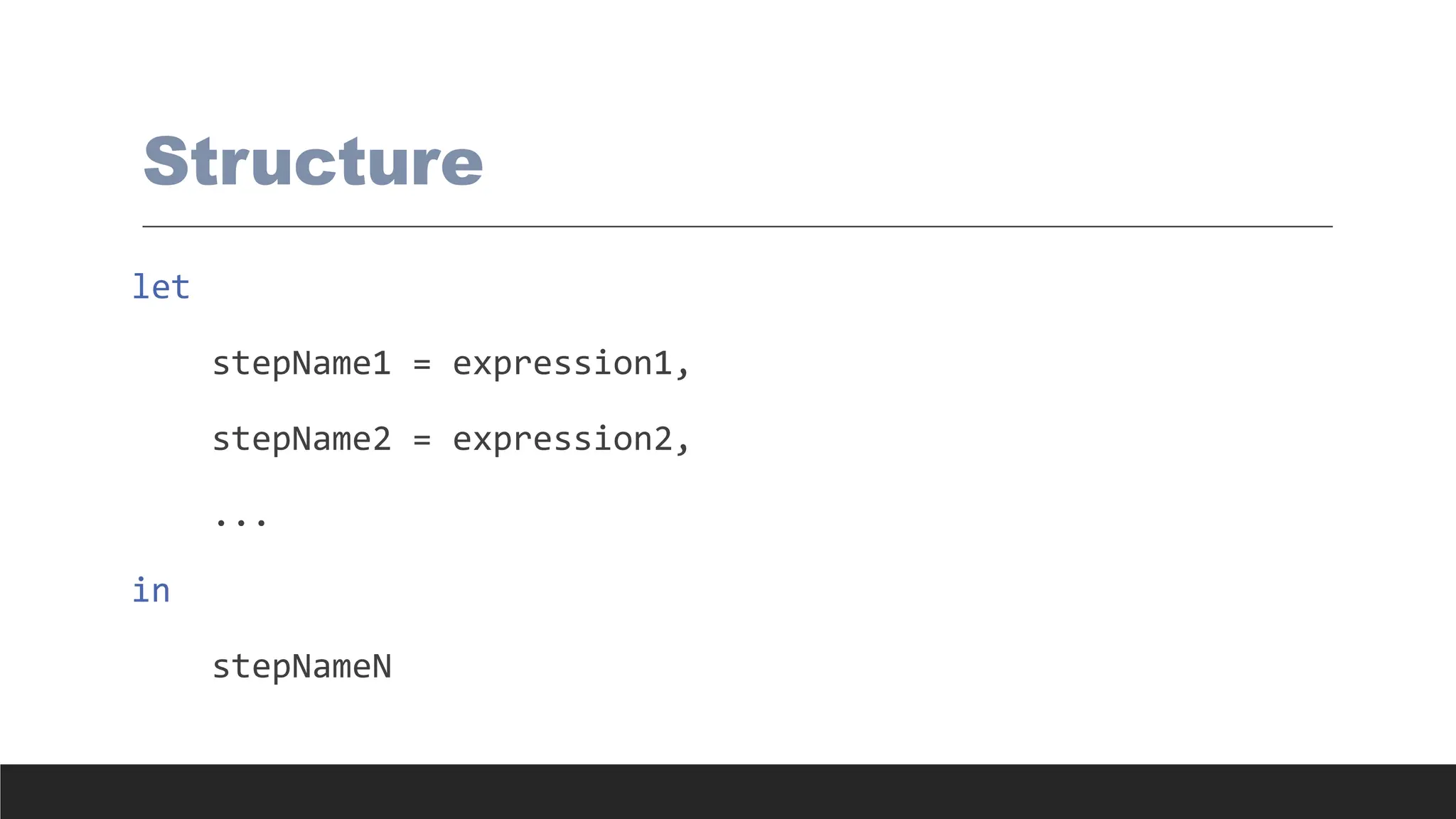
![Syntax
Rules
Concept Example
Comments // single line, /* block */
Variables myVar = 5
Lists {1, 2, 3}
Records [Name="Alice", Age=25]
Tables #table({"Col1", "Col2"}, {{1, "A"}, {2, "B"}})
Functions (x) => x + 1
Case-sensitive Column1 ≠ column1](https://image.slidesharecdn.com/2-250703033149-22abe271/75/Data-Retrieval-and-Preparation-Business-Analytics-pdf-210-2048.jpg)
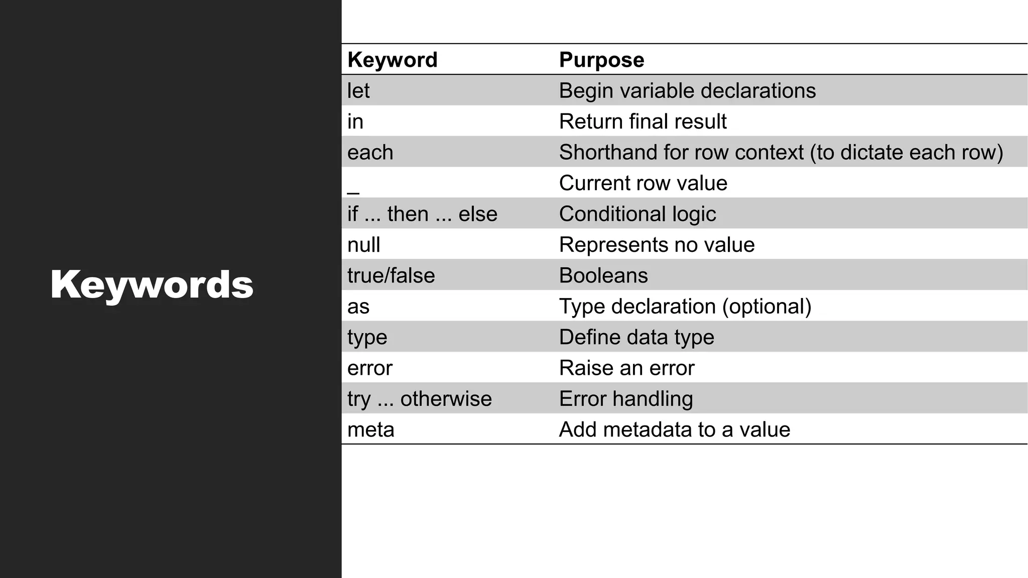

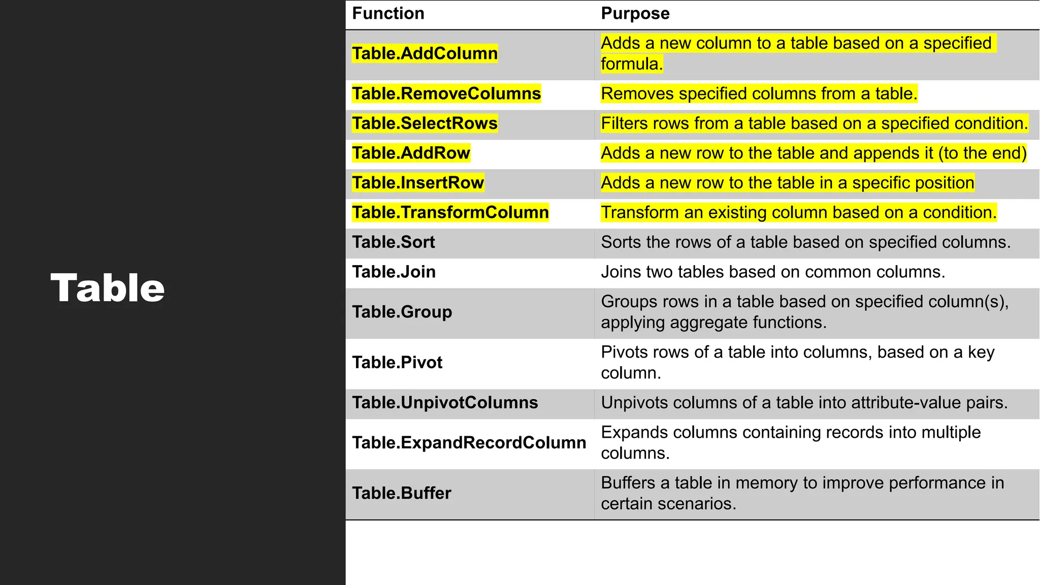
![Table Functions
> Table.SelectRows
◦ Table.SelectRows(table as table, condition as function) as table
◦ Table.SelectRows(SalesData, each [Amount] > 1000)
> Table.AddColumn
◦ Table.AddColumn(table as table, columnName as text, transformation as function) as
table
◦ Table.AddColumn(SalesData, "Discounted Price", each [Amount] * (1 -
[Discount]))
◦ Table.AddColumn(SalesData, "SalesLevel", each if [Amount] > 1000 then
"High" else "Low")](https://image.slidesharecdn.com/2-250703033149-22abe271/75/Data-Retrieval-and-Preparation-Business-Analytics-pdf-214-2048.jpg)
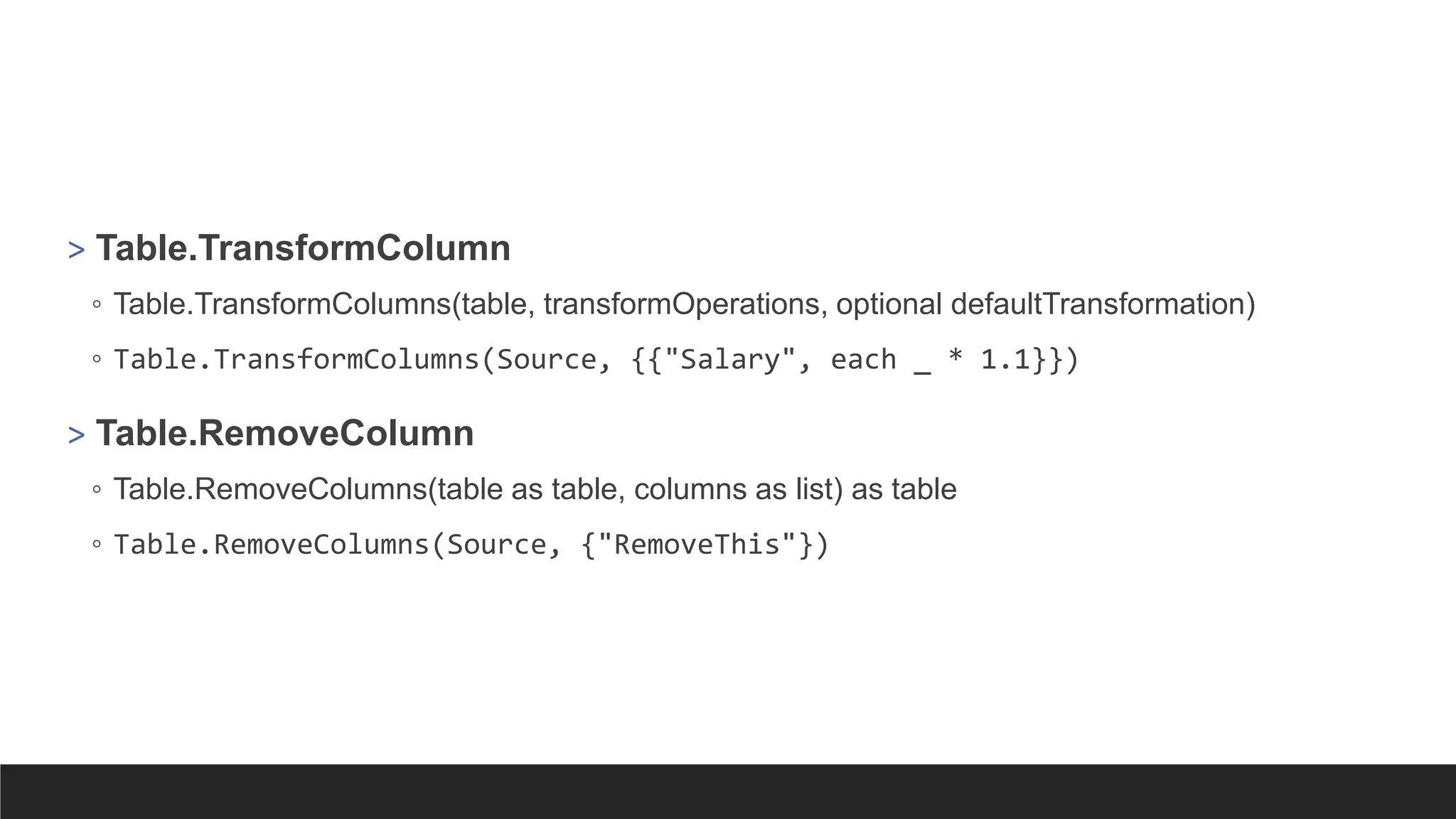
![> Table.AddRow
let
Source = Table.FromRecords({
[Name = "Alice", Age = 30],
[Name = "Bob", Age = 25]
}),
NewRow = [Name = "Charlie", Age = 35],
UpdatedTable = Table.AddRow(Source, NewRow)
in
UpdatedTable](https://image.slidesharecdn.com/2-250703033149-22abe271/75/Data-Retrieval-and-Preparation-Business-Analytics-pdf-216-2048.jpg)
![> Table.InsertRows
let
Source = Table.FromRecords({
[Name = "Alice", Age = 30],
[Name = "Bob", Age = 25]
}),
NewRow = [Name = "Charlie", Age = 35],
UpdatedTable = Table.InsertRows(Source, 2, {NewRow})
in
UpdatedTable](https://image.slidesharecdn.com/2-250703033149-22abe271/75/Data-Retrieval-and-Preparation-Business-Analytics-pdf-217-2048.jpg)
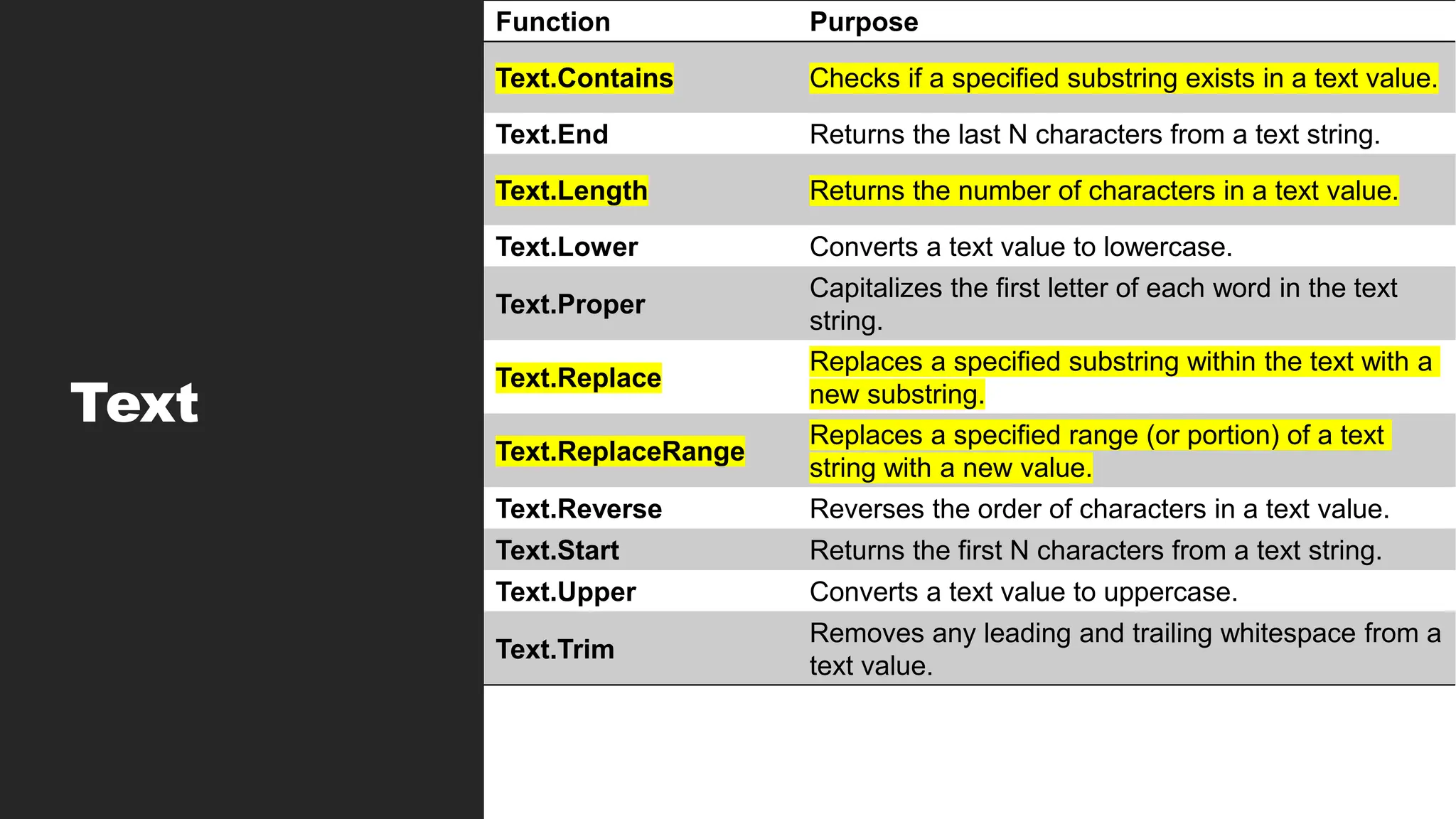
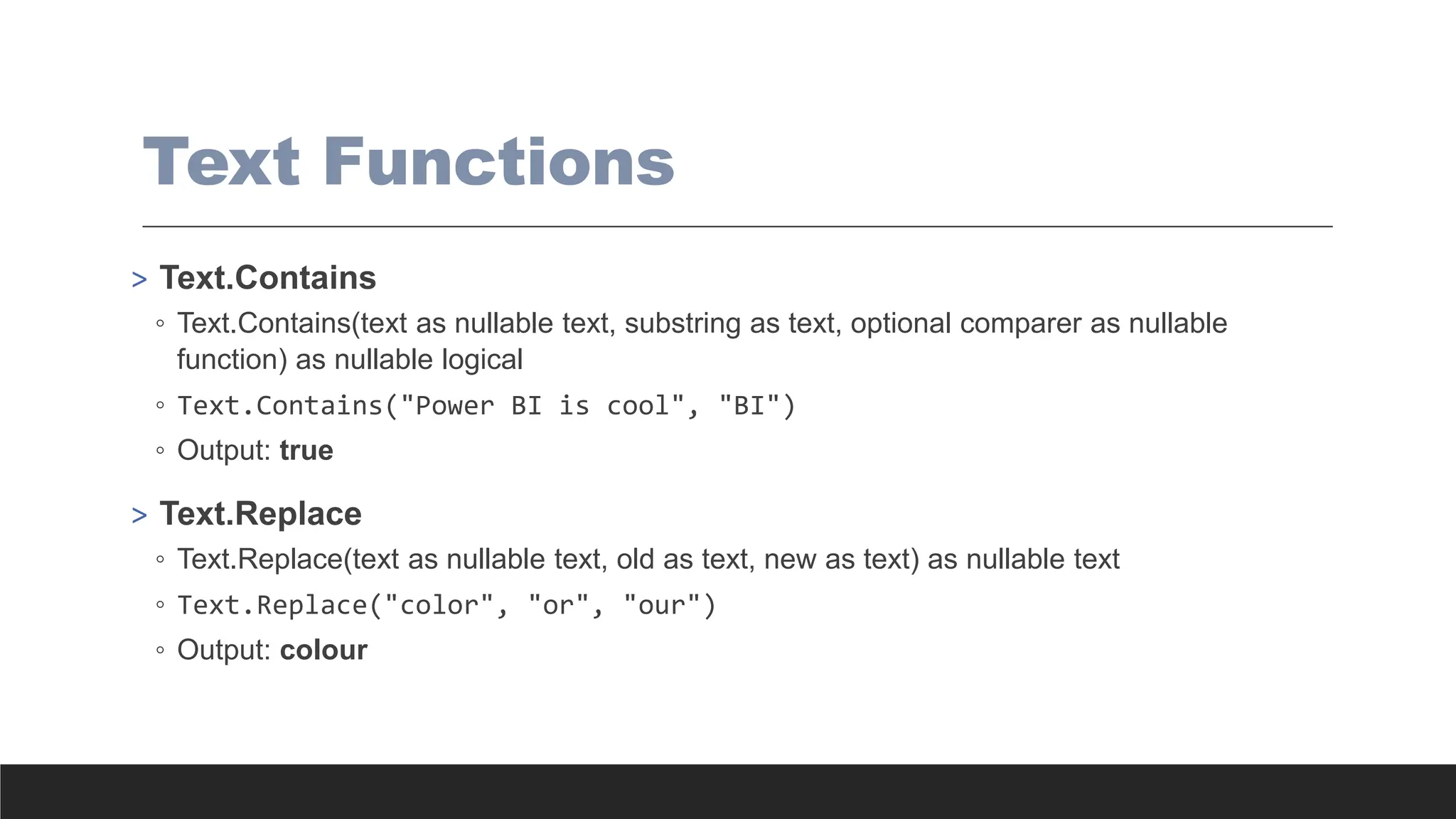
![> Text.ReplaceRange
◦ Text.ReplaceRange(text as text, offset as number, length as number, newText as text) as text
◦ Text.ReplaceRange("abcdef", 2, 3, "XYZ")
◦ Output: abXYZf
> Text.Replace with Conditions
◦ Table.TransformColumns(YourTable, {{"Product", each if [SalesAmount] > 1000
then Text.Replace(_, "Expensive", "Premium") else _, type text}})
◦ Output: For each sales greater than 1000, it replaces the value in Product (value of each
row represented with _ (underscore)) if the value is “Expensive” to “Premium”.
Otherwise keeps original value.](https://image.slidesharecdn.com/2-250703033149-22abe271/75/Data-Retrieval-and-Preparation-Business-Analytics-pdf-220-2048.jpg)

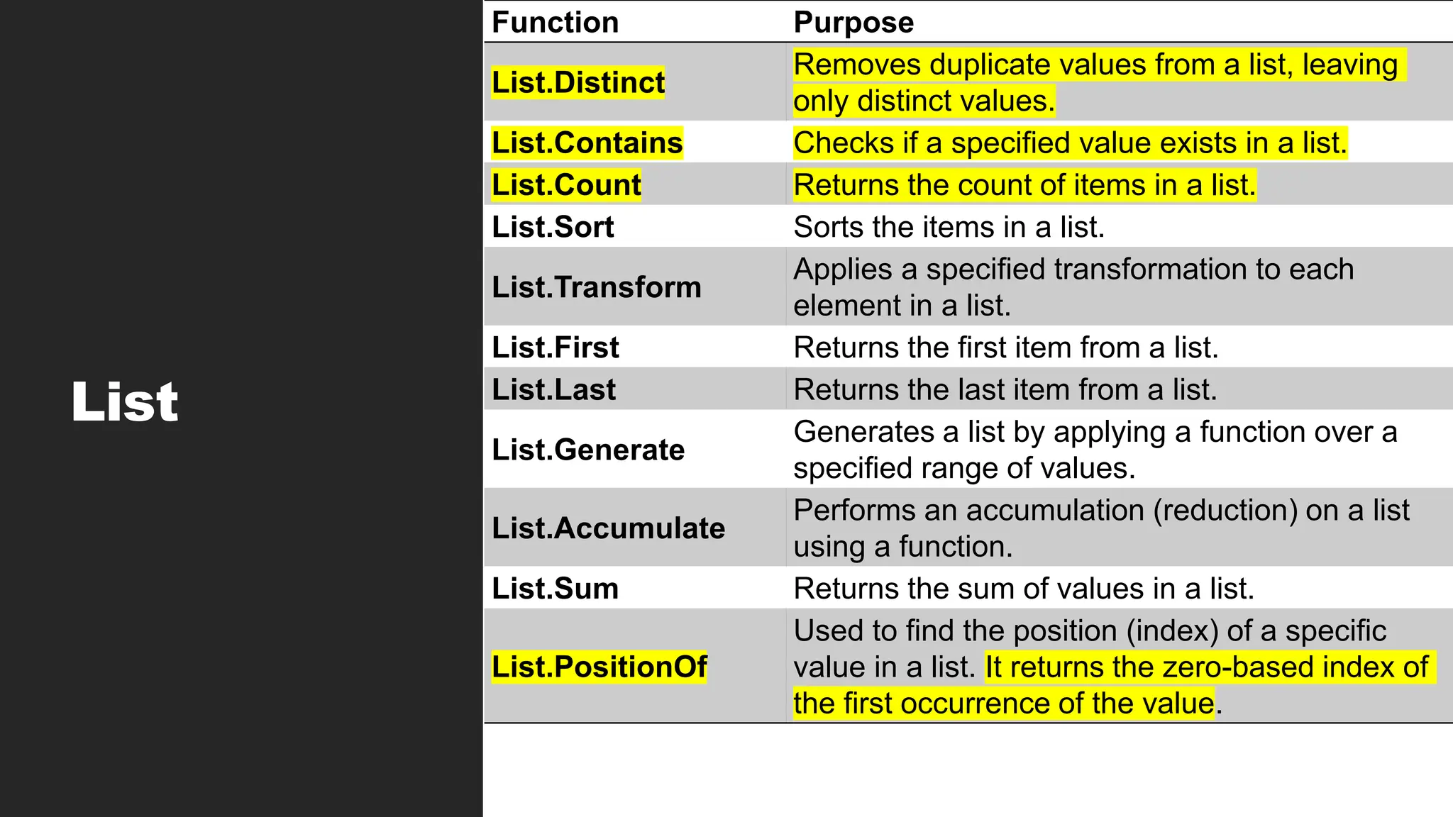
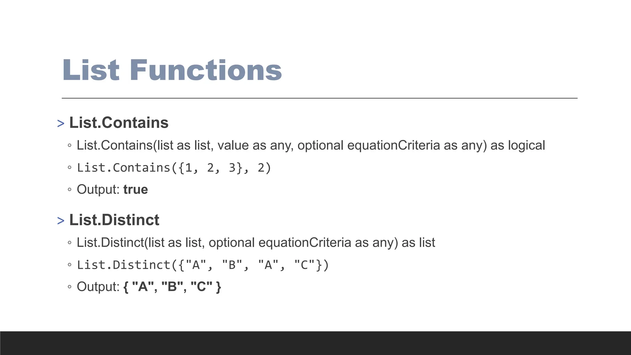
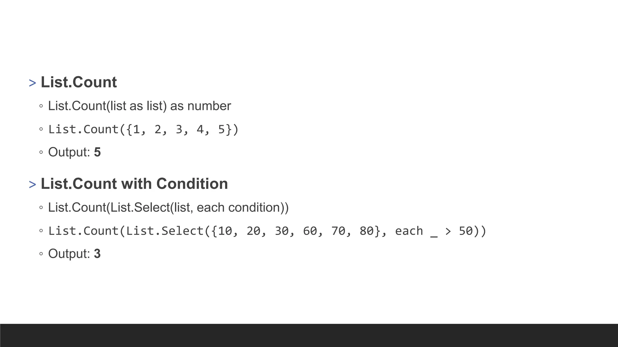
![Lookup with Custom Columns
> =Table[ColumnToReturn]{List.PositionOf(Table[ColumnToMatch],[ColumnToLook
Up])}
> =Categories[Category]{List.PositionOf(Categories[Acronym],[Cat])}
> This finds the position of [Cat] in Categories[Acronym], then returns
Categories[Category] from the same position. Similar to a Lookup.
> = Table.AddColumn(#“LastStep", "Category", each
Categories[Category]{List.PositionOf(Categories[Acronym],[Cat])})](https://image.slidesharecdn.com/2-250703033149-22abe271/75/Data-Retrieval-and-Preparation-Business-Analytics-pdf-225-2048.jpg)

![Count Distinct Values for Each
Group with M
= Table.Group(#"Changed Type", {"EmployeeID", "EmployeeName"}, {{"Total Sales",
each List.Sum([Total]), type nullable number},{"Number of Orders", each
List.Count(List.Distinct([OrderID])), type number}})](https://image.slidesharecdn.com/2-250703033149-22abe271/75/Data-Retrieval-and-Preparation-Business-Analytics-pdf-227-2048.jpg)
![Min-Max Normalization with
Custom Columns
> ([Column] - List.Min(#“Previous Step"[Sales]))/(List.Max(#" Previous Step "[Sales]) -
List.Min(#" Previous Step "[Sales]))
> ([Sales] - List.Min(#"Changed Type2"[Sales]))/(List.Max(#"Changed
Type2"[Sales]) - List.Min(#"Changed Type2"[Sales]))
> = Table.AddColumn(#"Changed Type2", "Normalized Sales", each ([Sales]
- List.Min(#"Changed Type2"[Sales]))/(List.Max(#"Changed
Type2"[Sales]) - List.Min(#"Changed Type2"[Sales])))](https://image.slidesharecdn.com/2-250703033149-22abe271/75/Data-Retrieval-and-Preparation-Business-Analytics-pdf-228-2048.jpg)
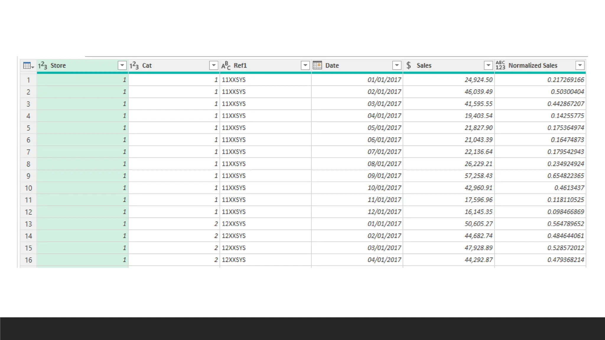
![Z-Value Normalization with
Custom Columns
> ([Column]-List.Average(#“Previous Step"[Column]))/(List.StandardDeviation(#“Previous
Step"[Column]))
> ([Sales]-List.Average(#"Added
Custom"[Sales]))/(List.StandardDeviation(#"Added Custom"[Sales]))
> = Table.AddColumn(#"Added Custom", "Z-Value Normalized Sales", each
([Sales]-List.Average(#"Added
Custom"[Sales]))/(List.StandardDeviation(#"Added Custom"[Sales])))](https://image.slidesharecdn.com/2-250703033149-22abe271/75/Data-Retrieval-and-Preparation-Business-Analytics-pdf-230-2048.jpg)
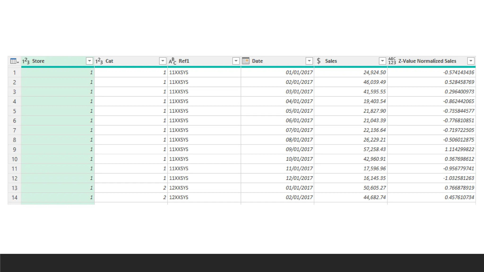
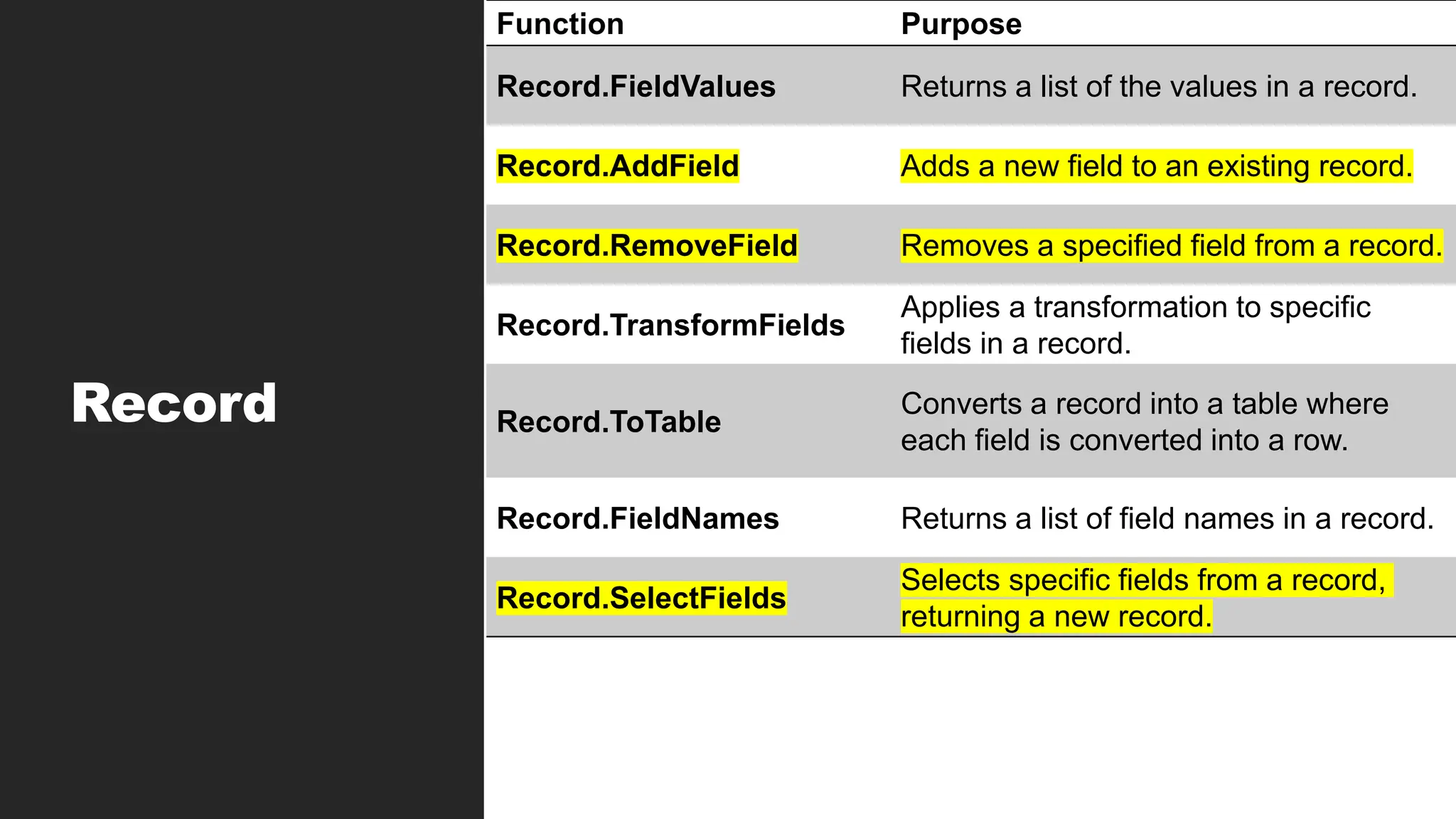
![Record Function
> Record.AddField
◦ Record.AddField(record as record, fieldName as text, fieldValue as any) as record
◦ Record.AddField([Name = "Alice", Age = 30], "LoyaltyStatus", "Gold")
◦ Output: [Name = "Alice", Age = 30, LoyaltyStatus = "Gold"]
> Record.SelectFields
◦ Record.SelectFields(record as record, fieldNames as list) as record
◦ Record.SelectFields([Name = "Alice", Age = 30, Address = "123 Maple
St"], {"Name", "Age"})
◦ Output: [Name = "Alice", Age = 30]](https://image.slidesharecdn.com/2-250703033149-22abe271/75/Data-Retrieval-and-Preparation-Business-Analytics-pdf-233-2048.jpg)
![> Record.RemoveField
◦ Record.RemoveField(record as record, fieldName as text) as record
◦ Record.RemoveField([Name = "Alice", Age = 30, Address = "123 Maple St"],
"Address")
◦ Output: [Name = "Alice", Age = 30]](https://image.slidesharecdn.com/2-250703033149-22abe271/75/Data-Retrieval-and-Preparation-Business-Analytics-pdf-234-2048.jpg)

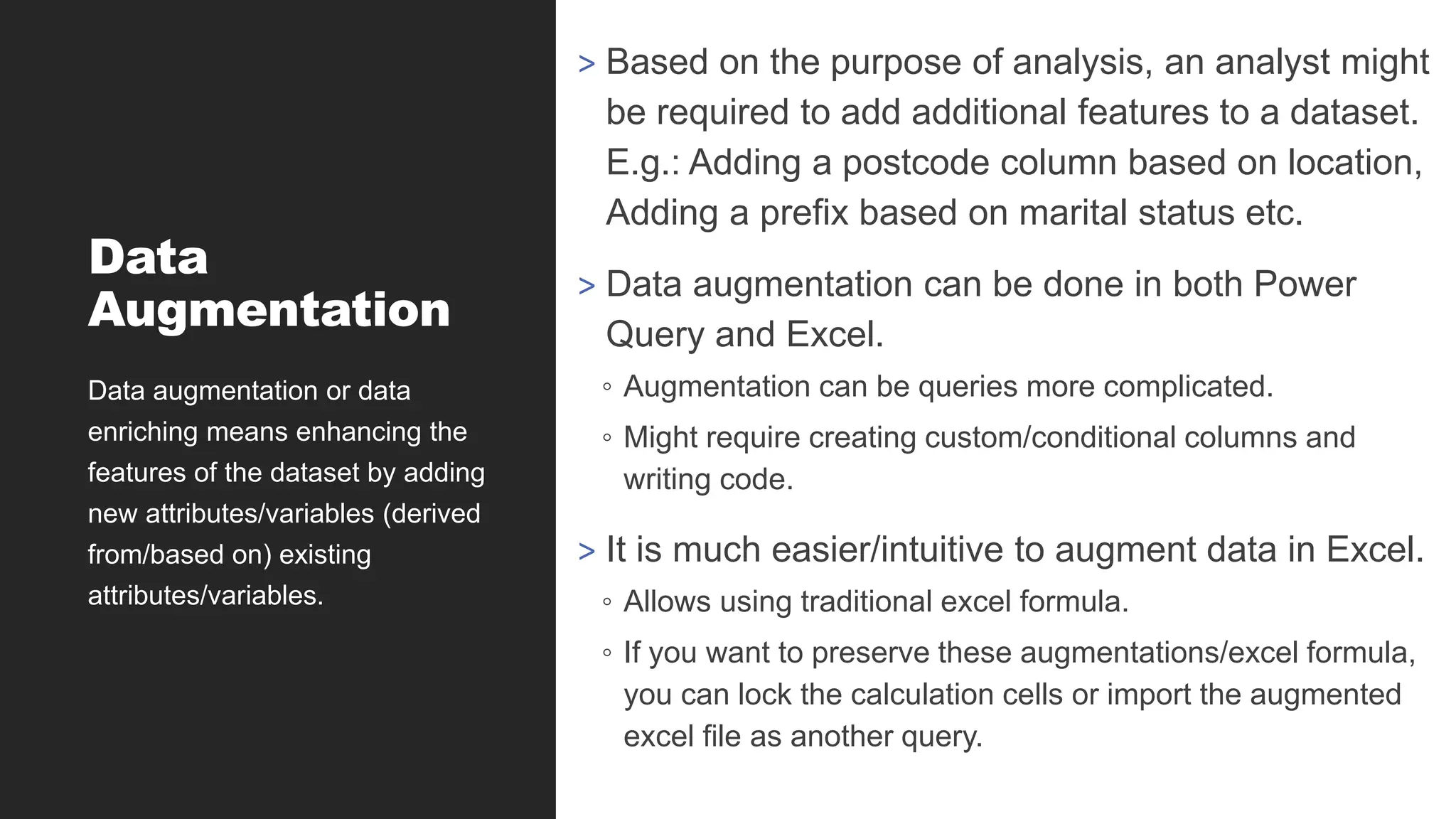

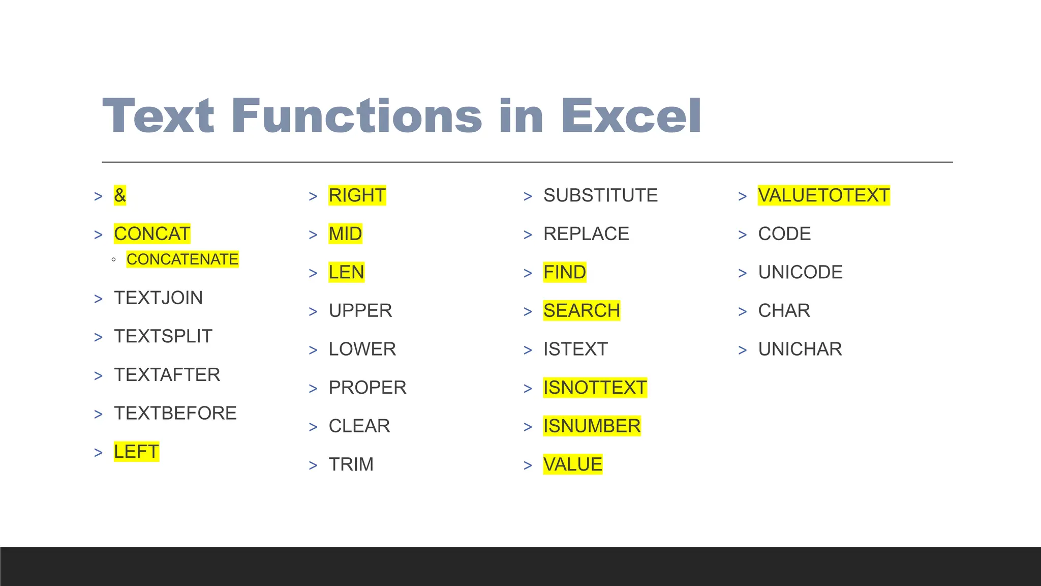
![Combine Data
> =CONCAT(text1, [text2]…)
> =TEXTJOIN(delimiter, ignore_empty, text1, [text2]…)
> & Operator (all cells must be selected individually to join)](https://image.slidesharecdn.com/2-250703033149-22abe271/75/Data-Retrieval-and-Preparation-Business-Analytics-pdf-243-2048.jpg)
![Split Data
> =LEFT(text, [num_chars])
> =RIGHT(text, [num_chars])
> =MID(text, start_num, [num_chars])](https://image.slidesharecdn.com/2-250703033149-22abe271/75/Data-Retrieval-and-Preparation-Business-Analytics-pdf-244-2048.jpg)
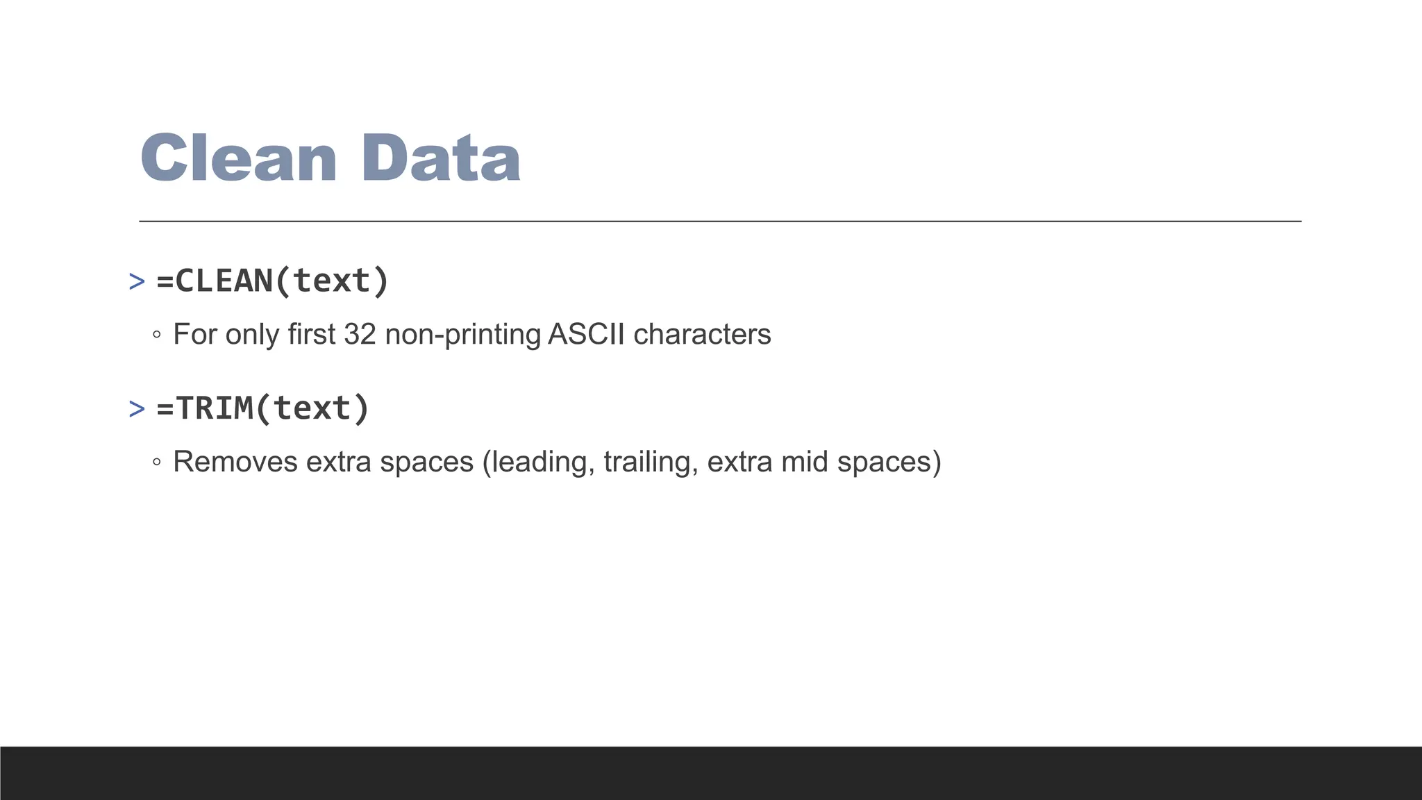
![Modify/Replace Data
> =LEN(text)
> =FIND(find_text, within_text, [start_num])
> =UPPER(text)
> =LOWER(text)
> =PROPER(text)
> =SUBSTITUTE(text, old_text, new_text, [instance_num])
> =VALUE(text)](https://image.slidesharecdn.com/2-250703033149-22abe271/75/Data-Retrieval-and-Preparation-Business-Analytics-pdf-246-2048.jpg)
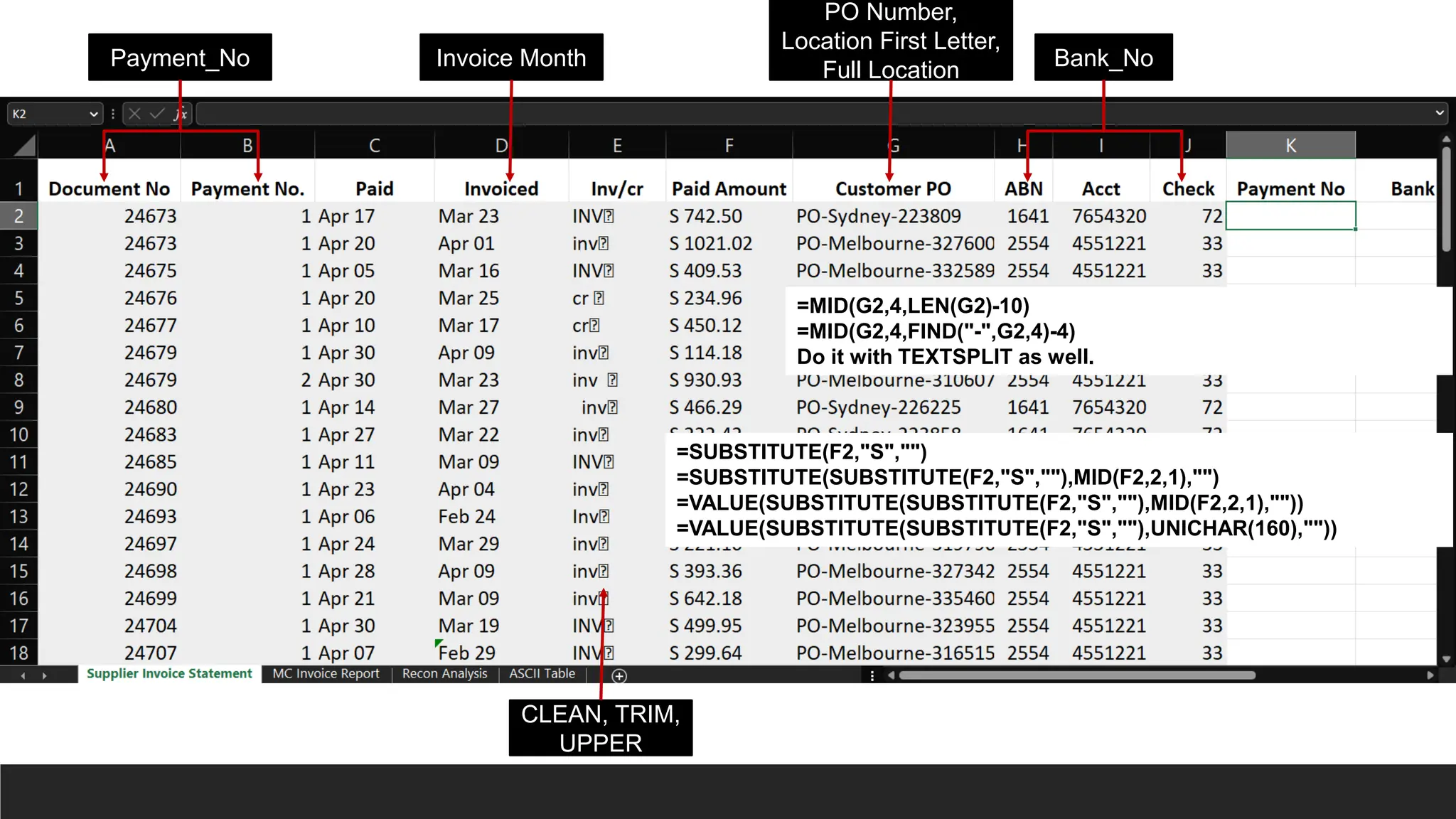

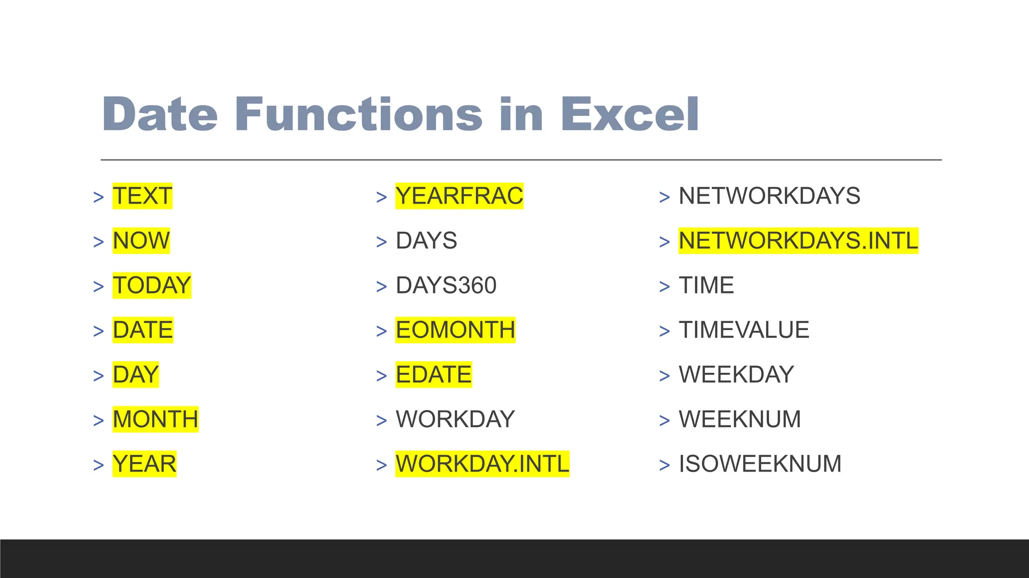
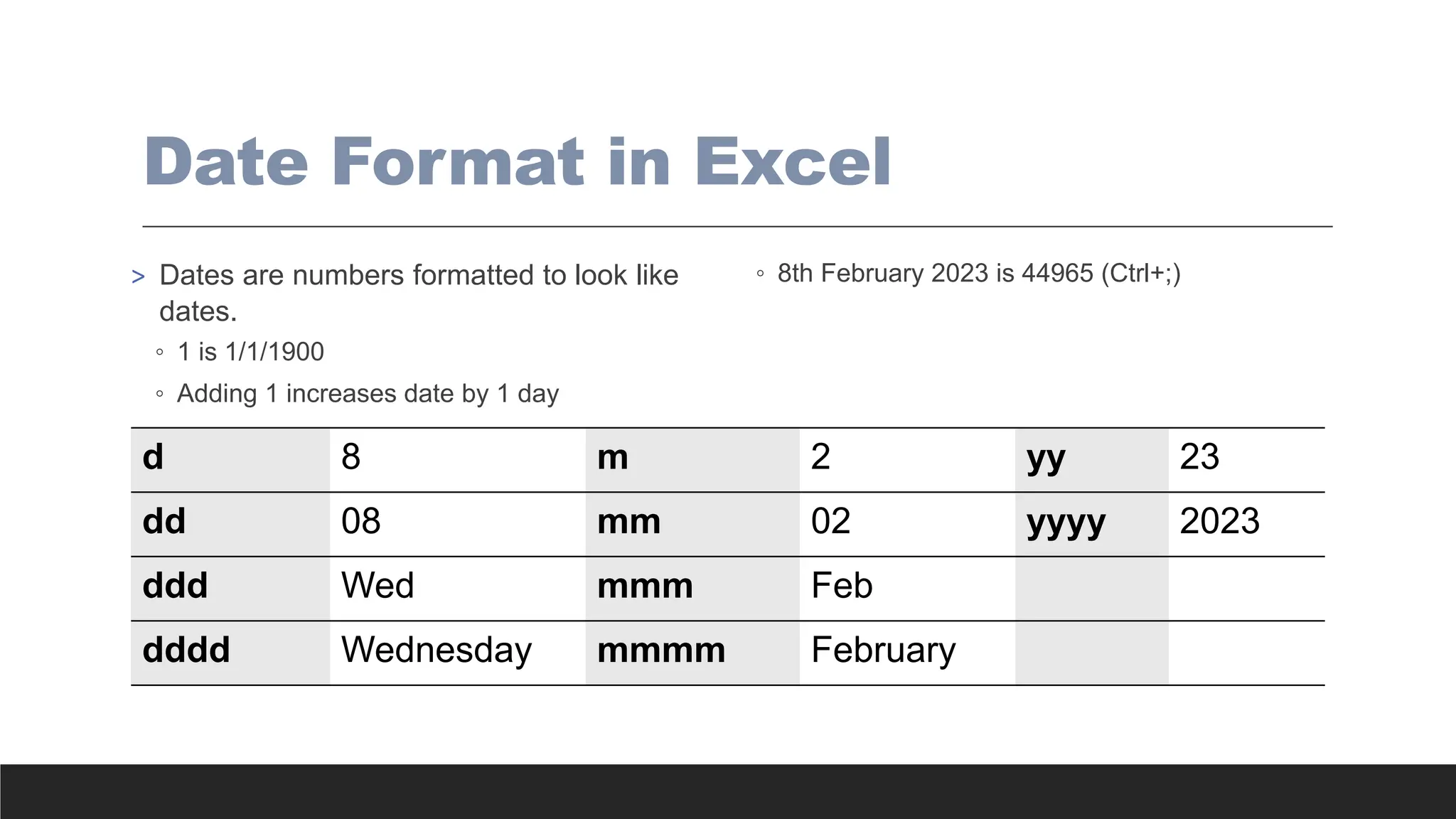
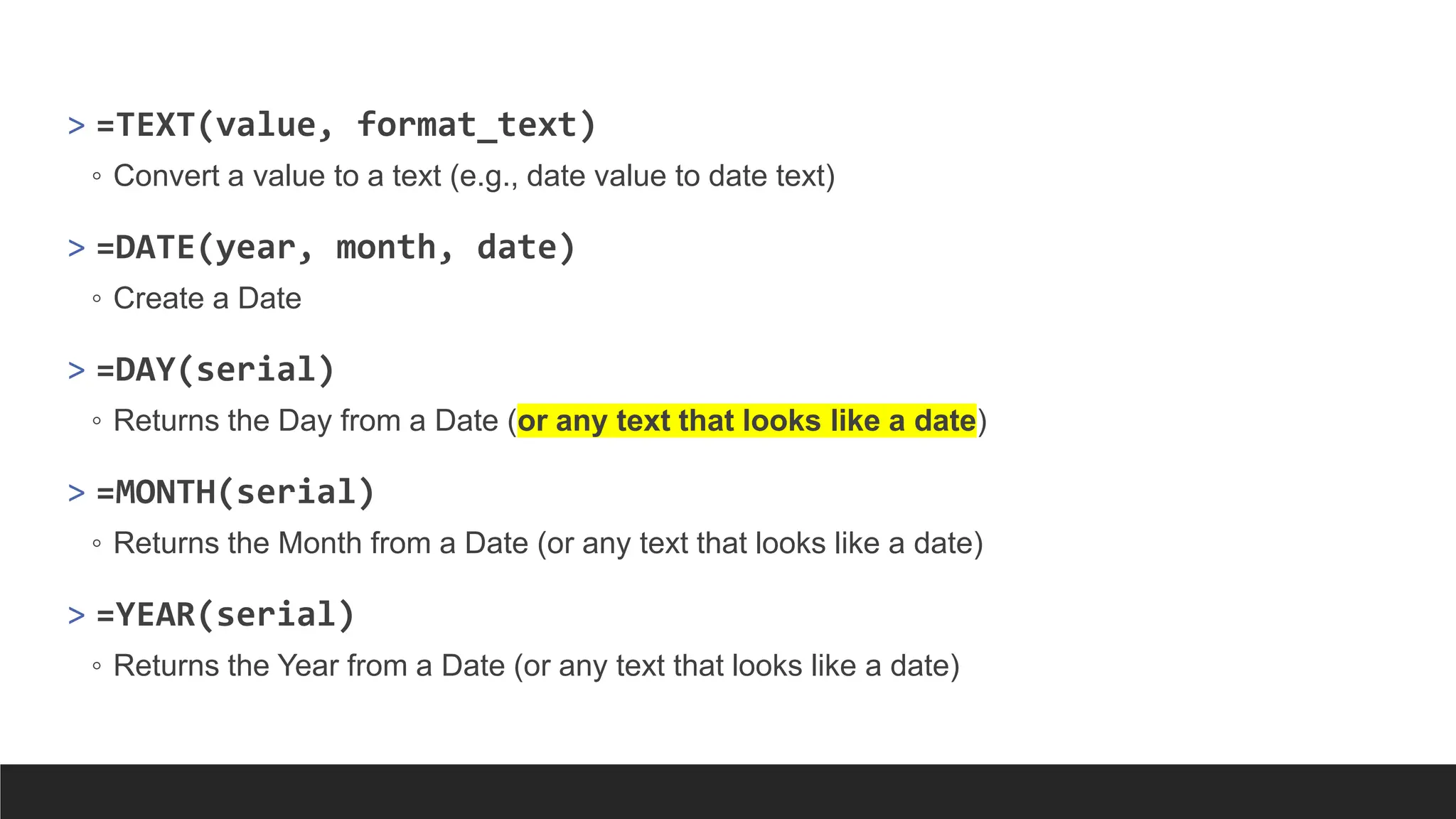
![> =EOMONTH(start_date, months)
◦ Find the last day of a month a certain number of months before or after a given date.
> =EDATE(start_date, months)
◦ Move a certain number of months before or after a given date.
> =YEARFRAC(start_date, end_date, [basis])
◦ Returns the year fraction representing the number of days between start date & end date.
> =DAYS(end_date, start_date)
◦ Returns the number of days between two dates
> =DAYS360(end_date, start_date)
◦ Returns the number of days between two dates based on a 360 Day year (12, 30-day monts)](https://image.slidesharecdn.com/2-250703033149-22abe271/75/Data-Retrieval-and-Preparation-Business-Analytics-pdf-252-2048.jpg)
![> =WORKDAY(start_date, days, [holidays])
◦ Find the next workday before or after a given date. This excludes weekends and holidays. Saturday
& Sunday weekends. (days argument must be at least 1)
> =WORKDAY.INTL(start_date, days, [weekend], [holidays])
◦ Find the next workday before or after a given date. This excludes weekends and holidays. You can
specify the weekend dates as well. E.g., “0000110” – Friday, Saturday weekend.
> =NETWORKDAYS(start_date, end_date, [holidays])
◦ Find the number of workdays between 2 dates. This excludes weekends and holidays. Saturday &
Sunday weekends.
> =NETWORKDAYS.INTL(start_date, end_date, [weekend], [holidays])
◦ Find the number of workdays between 2 dates. This excludes weekends and holidays. You can
specify the weekend dates as well.](https://image.slidesharecdn.com/2-250703033149-22abe271/75/Data-Retrieval-and-Preparation-Business-Analytics-pdf-253-2048.jpg)
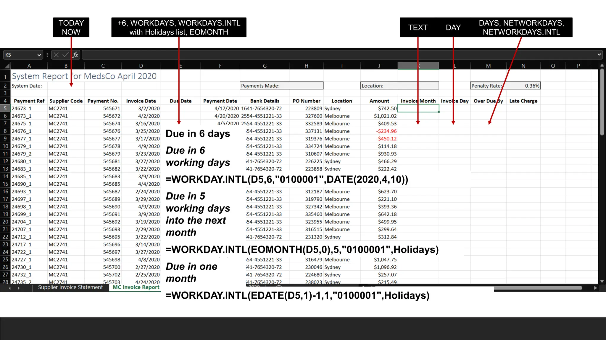
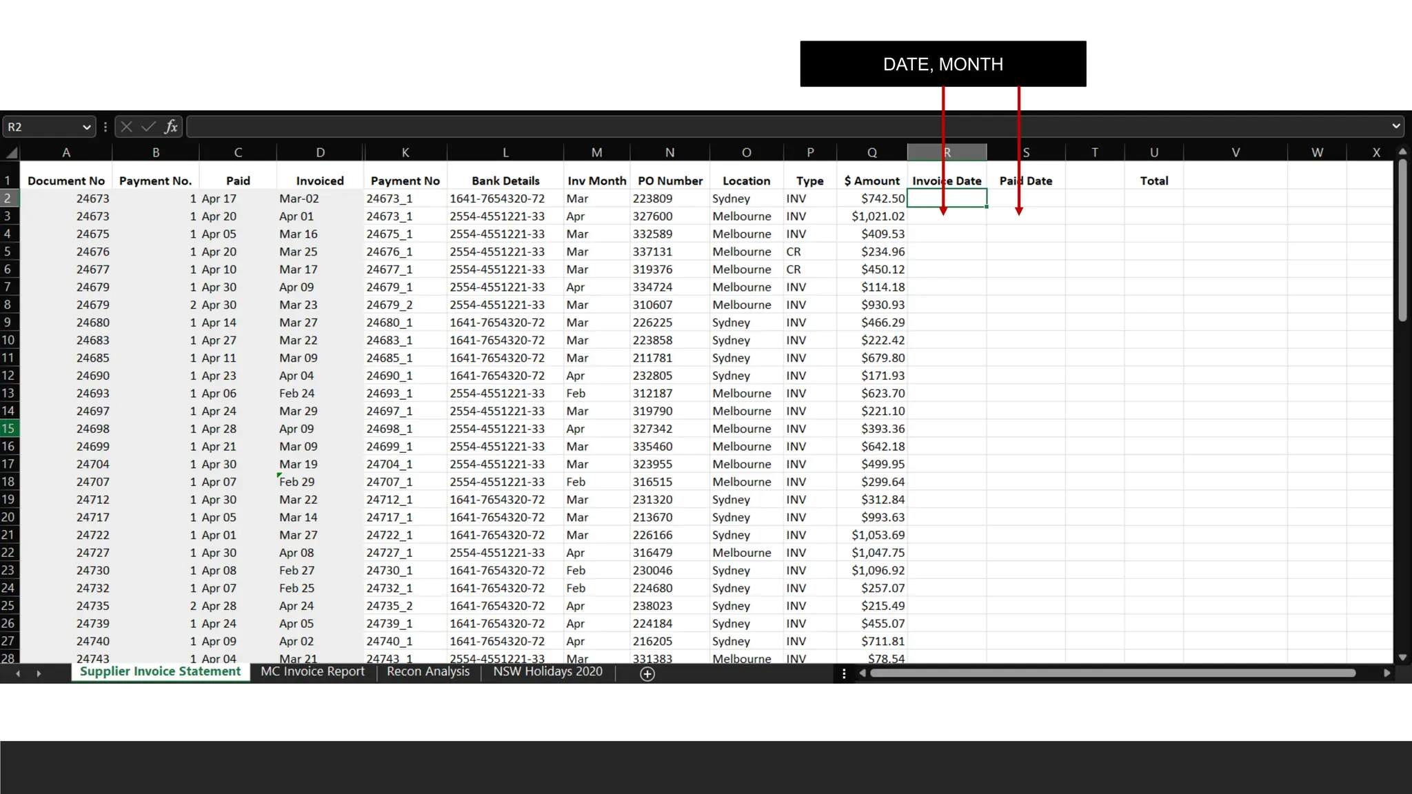
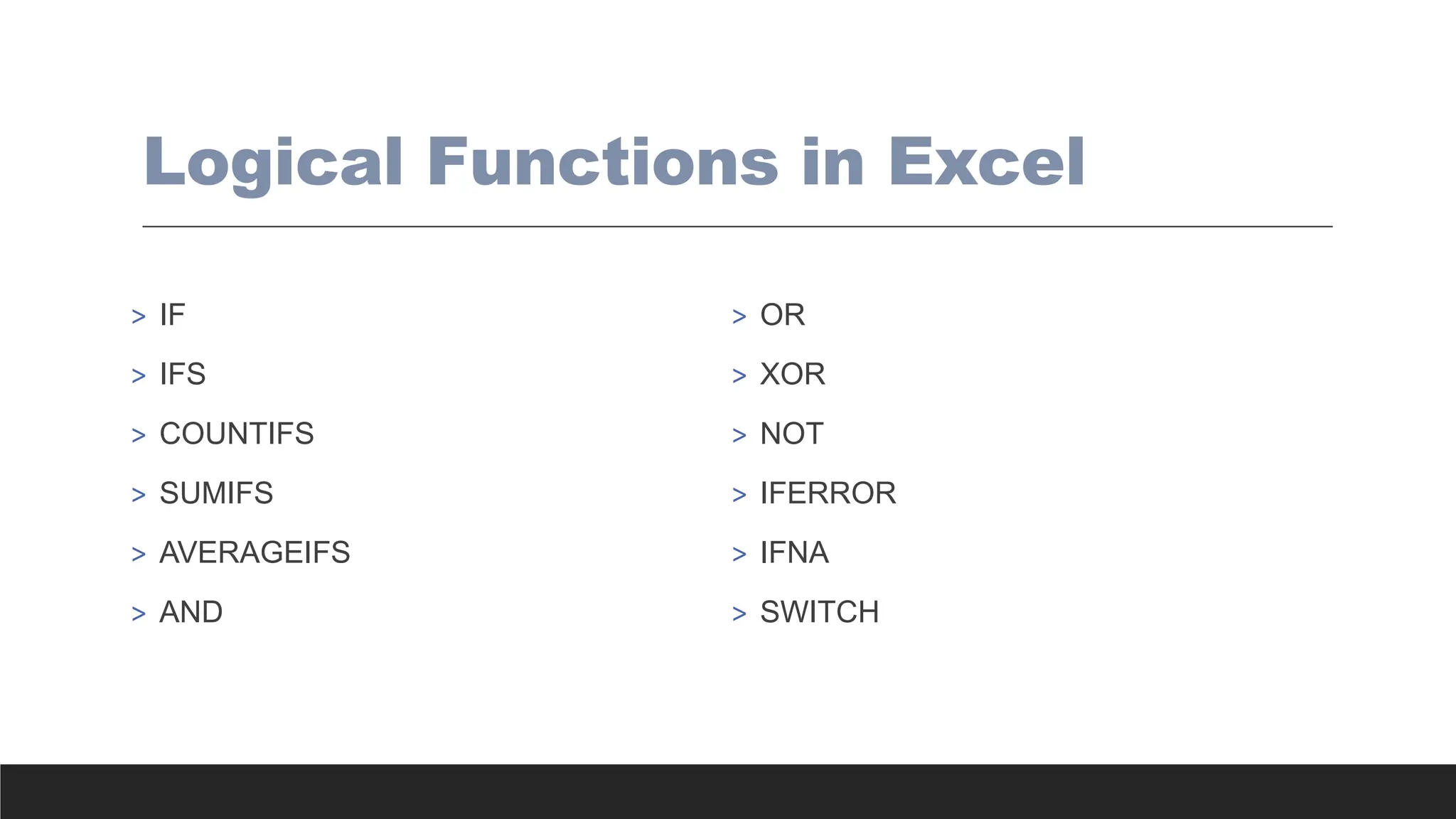
![IF
> The IF function is a premade function in Excel, which returns values based on
a true or false condition.
> It is typed =IF and has 3 parts:
◦ =IF(logical_test, [value_if_true], [value_if_false])
◦ Logical_test (required argument) – This is the condition to be tested and evaluated as
either TRUE or FALSE.
◦ Value_if_true (optional argument) – The value that will be returned if the logical_test
evaluates to TRUE.
◦ Value_if_false (optional argument) – The value that will be returned if the logical_test
evaluates to FALSE](https://image.slidesharecdn.com/2-250703033149-22abe271/75/Data-Retrieval-and-Preparation-Business-Analytics-pdf-258-2048.jpg)
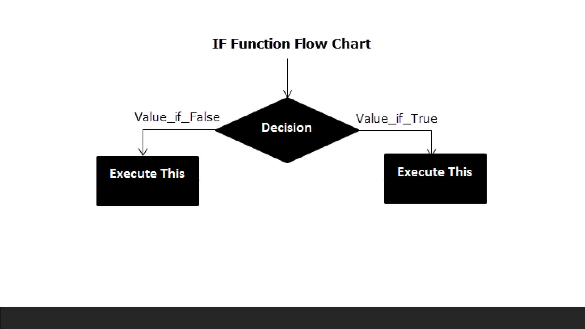
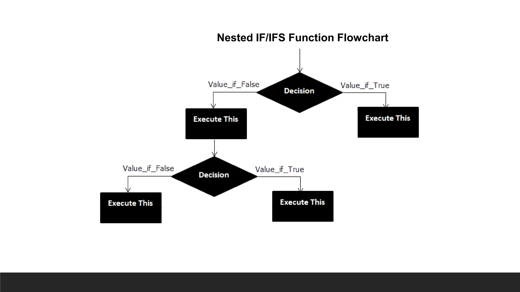
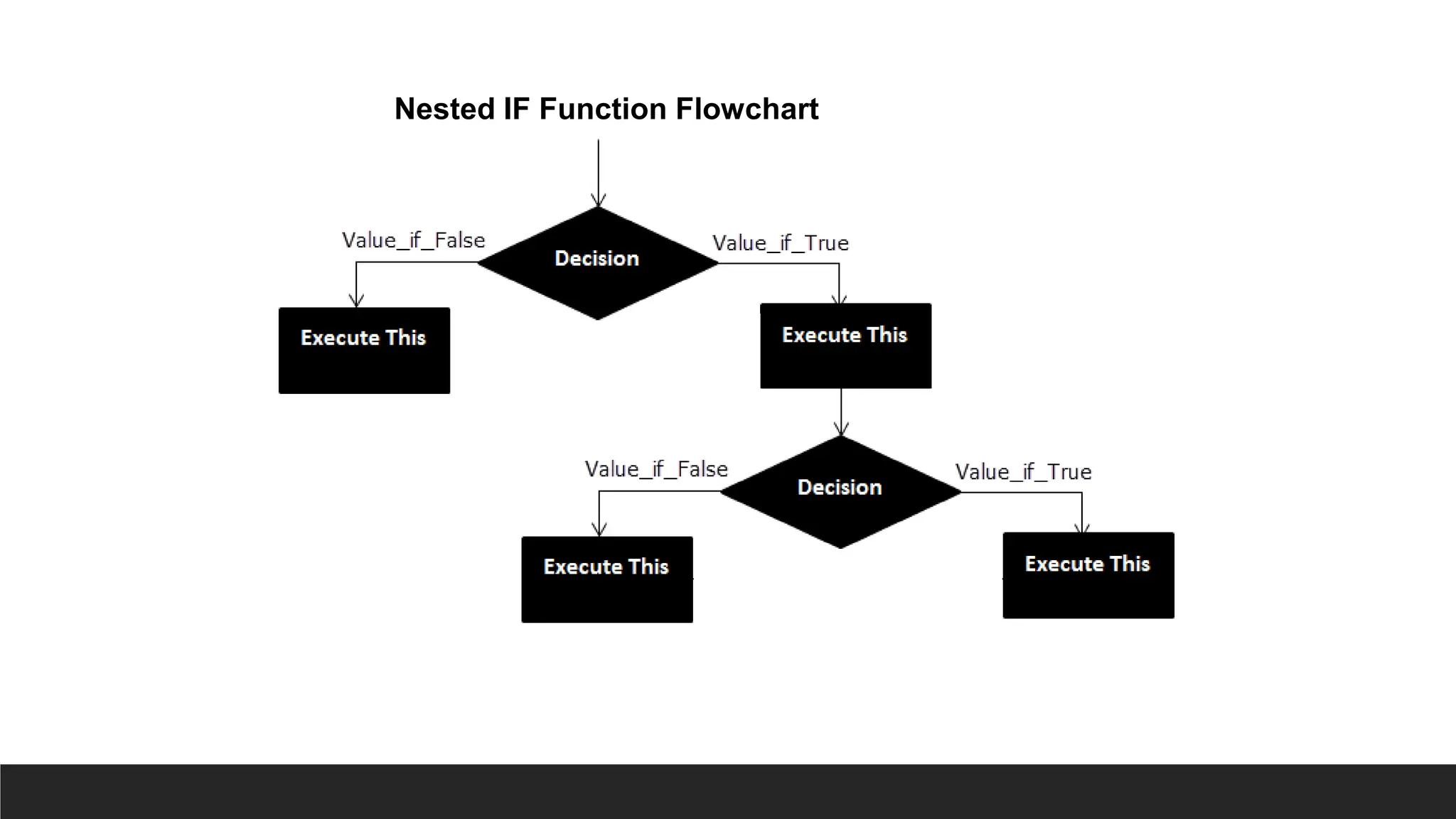

![Nested IF IFS
> The IFS function is a premade function in Excel, which returns values
based on one or more true or false conditions.
> It is typed =IFS and has two or more parts:
◦ =IFS(logical_test1, value_if_true1, [logical_test2, value_if_true2],
[logical_test3; ...)
◦ The conditions are referred to as logical_test1, logical_test2, ...
◦ Each condition relates to a return value.](https://image.slidesharecdn.com/2-250703033149-22abe271/75/Data-Retrieval-and-Preparation-Business-Analytics-pdf-263-2048.jpg)
![COUNTIFS
> The COUNTIFS function is a premade function in Excel, which counts
cells in a range based on one or more true or false condition.
> It is typed =COUNTIFS:
◦ =COUNTIFS(criteria_range1, criteria1, [criteria_range2, criteria2],
...)
◦ The conditions are referred to as critera1, criteria2, .. and so on
◦ The criteria_range1, criteria_range2, and so on, are the ranges where the
function check for the conditions.](https://image.slidesharecdn.com/2-250703033149-22abe271/75/Data-Retrieval-and-Preparation-Business-Analytics-pdf-264-2048.jpg)
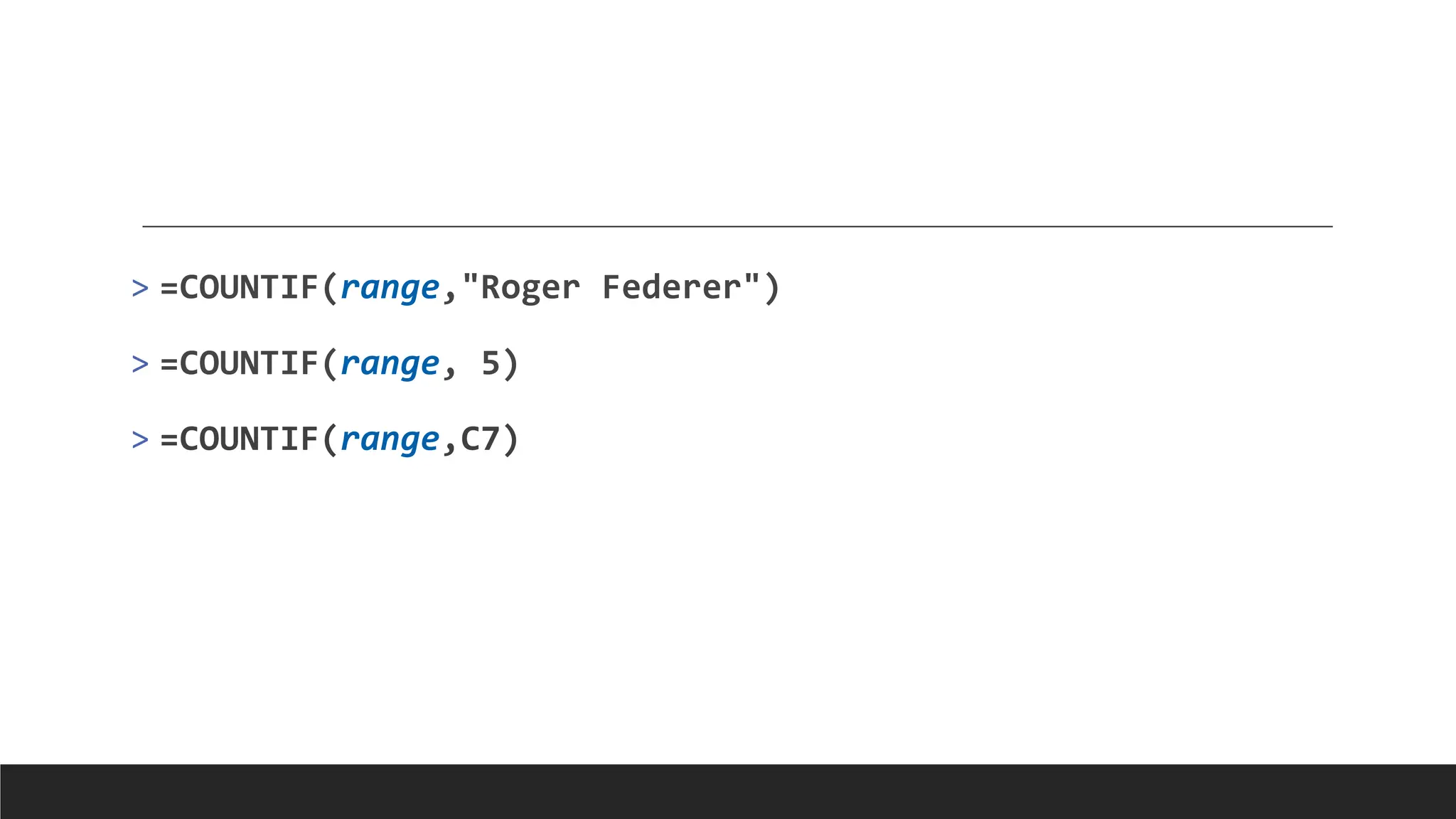
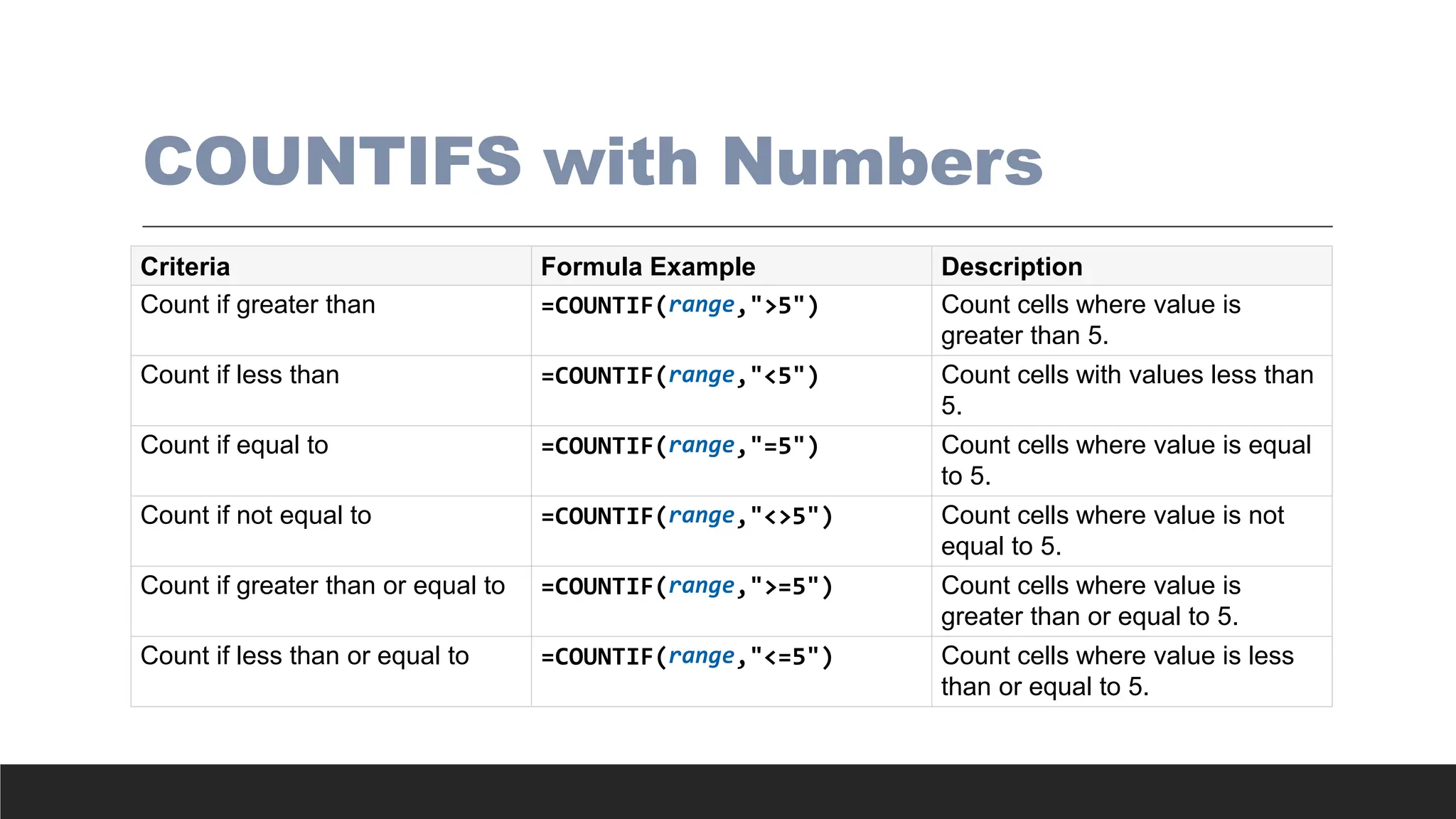
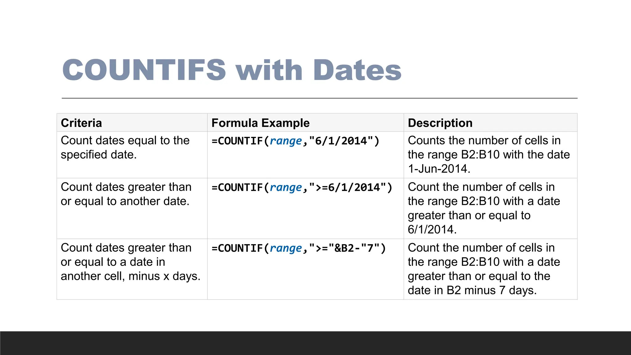
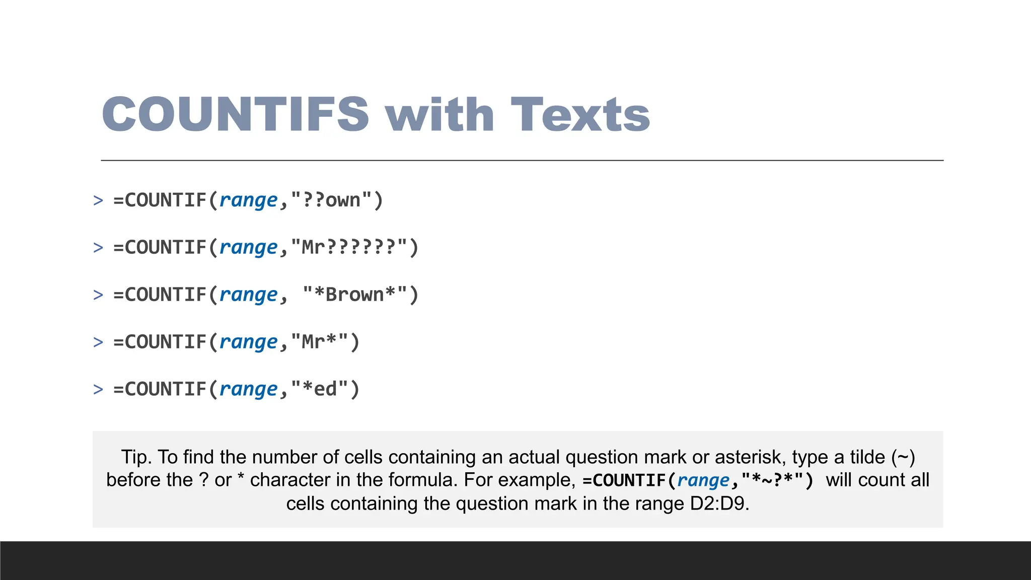
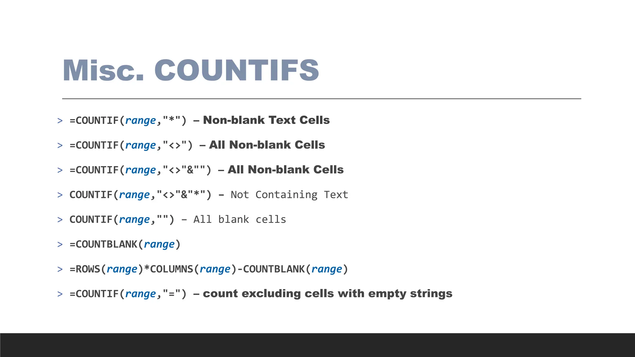
![SUMIFS
> The SUMIFS function is a premade function in Excel, which calculates
the sum of a range based on one or more true or false condition.
> It is typed =SUMIFS:
◦ =SUMIFS(sum_range, criteria_range1, criteria1, [criteria_range2,
criteria2] ...)
◦ The conditions are referred to as criteria1, criteria2, and so on.
◦ The [sum_range] is the range where the function calculates the sum.](https://image.slidesharecdn.com/2-250703033149-22abe271/75/Data-Retrieval-and-Preparation-Business-Analytics-pdf-270-2048.jpg)
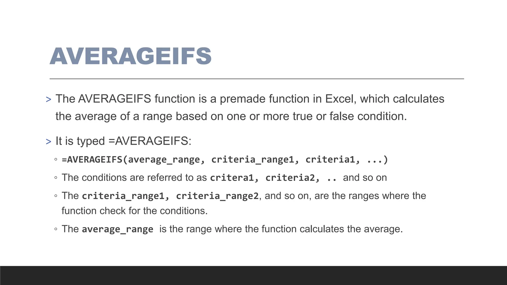
![AND
> The AND function is a premade function in Excel, which returns TRUE or
FALSE based on two or more conditions.
> It is typed =AND and takes two or more conditions.
◦ =AND([logical1], [logical2], ...)
◦ The conditions are referred to as [logical1], [logical2], and so on.](https://image.slidesharecdn.com/2-250703033149-22abe271/75/Data-Retrieval-and-Preparation-Business-Analytics-pdf-272-2048.jpg)
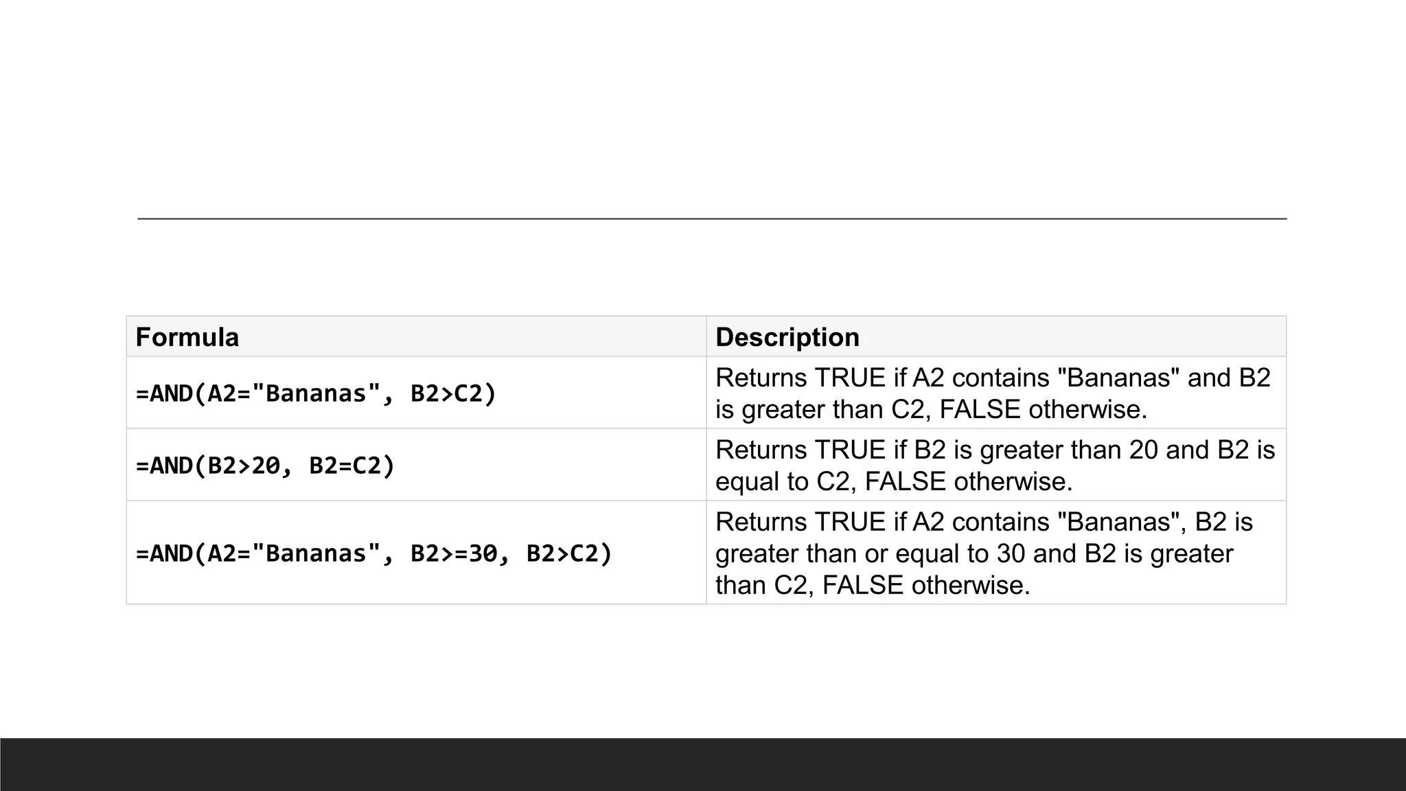
![OR
> The OR function is a premade function in Excel, which returns TRUE or
FALSE based on two or more conditions.
> It is typed =OR.
◦ =OR([logical1], [logical2], ...)
◦ The conditions are referred to as [logical1], [logical2], and so on.](https://image.slidesharecdn.com/2-250703033149-22abe271/75/Data-Retrieval-and-Preparation-Business-Analytics-pdf-274-2048.jpg)
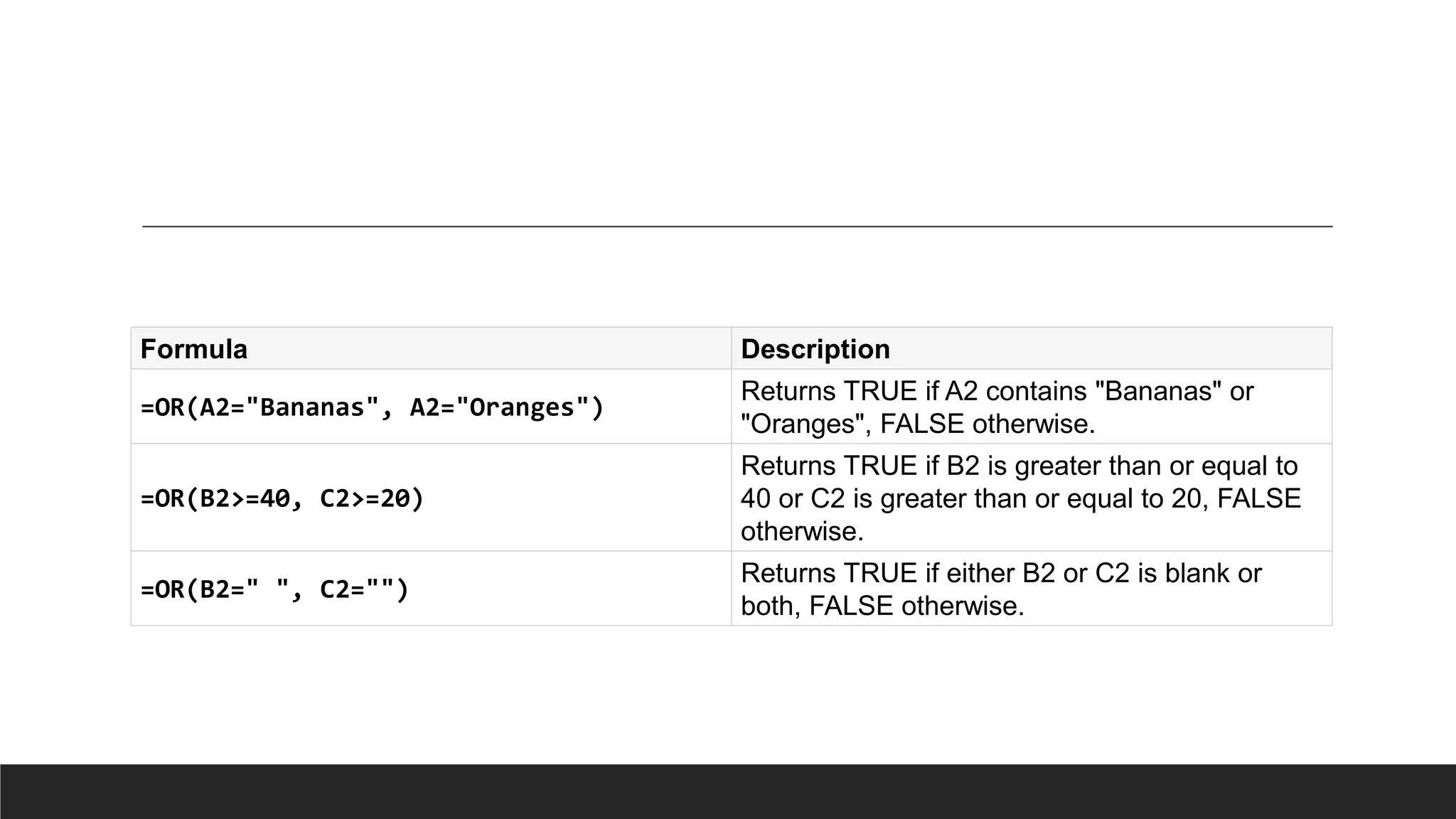
![XOR
> The XOR in Excel, which returns TRUE only if one of the conditions are
met.
> It is typed =XOR.
◦ =XOR([logical1], [logical2], ...)
◦ The conditions are referred to as [logical1], [logical2], and so on.
◦ TRUE if either argument evaluates to TRUE.
◦ FALSE if both arguments are TRUE or neither is TRUE.](https://image.slidesharecdn.com/2-250703033149-22abe271/75/Data-Retrieval-and-Preparation-Business-Analytics-pdf-276-2048.jpg)
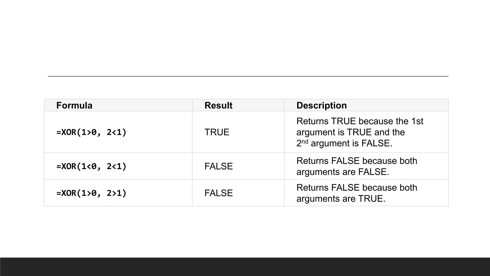
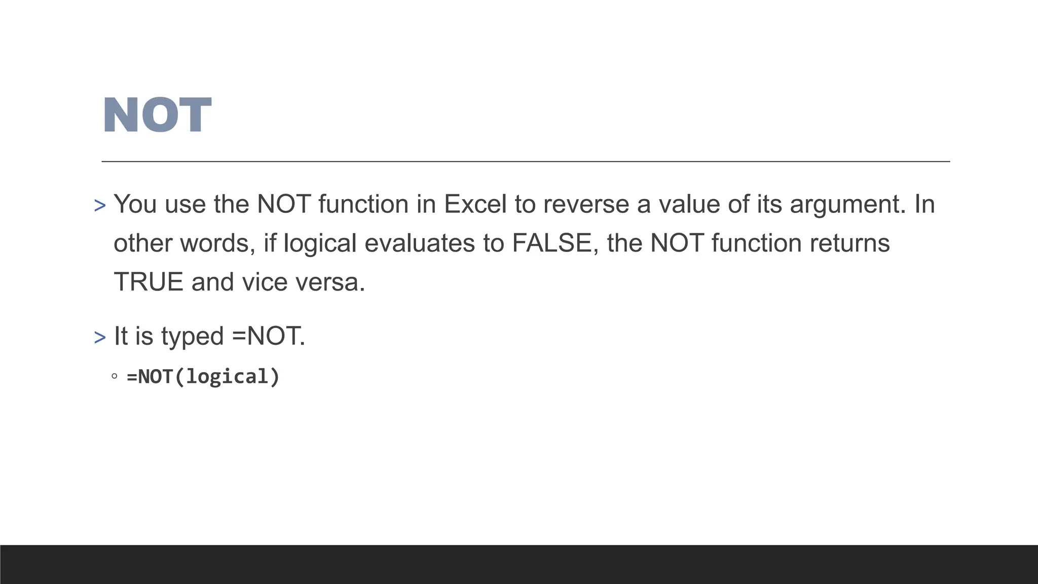
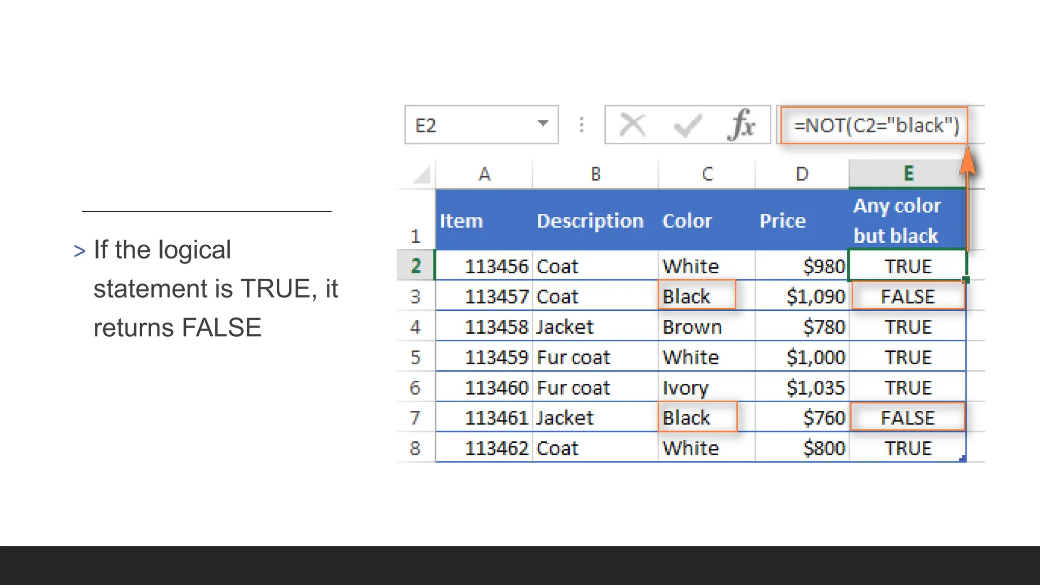
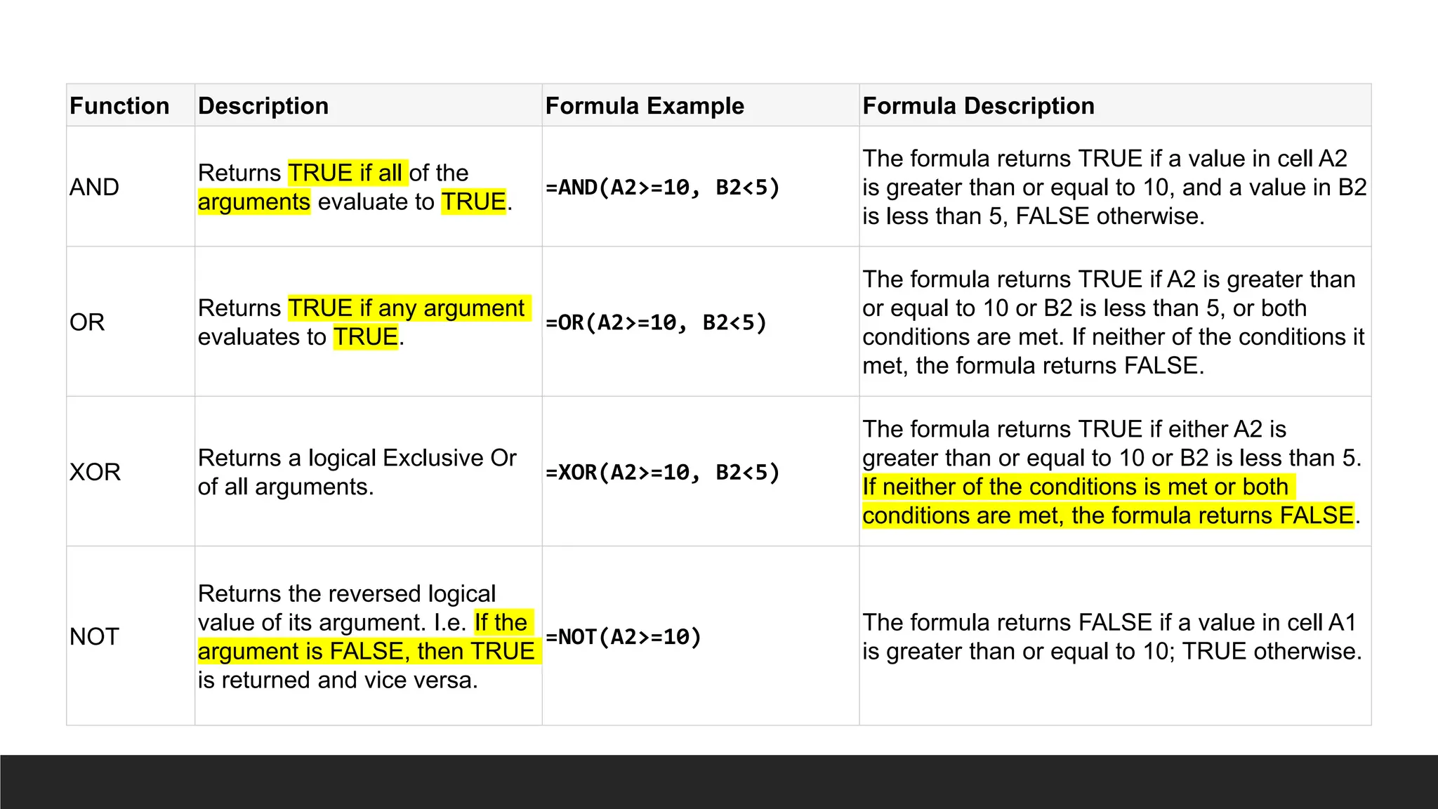
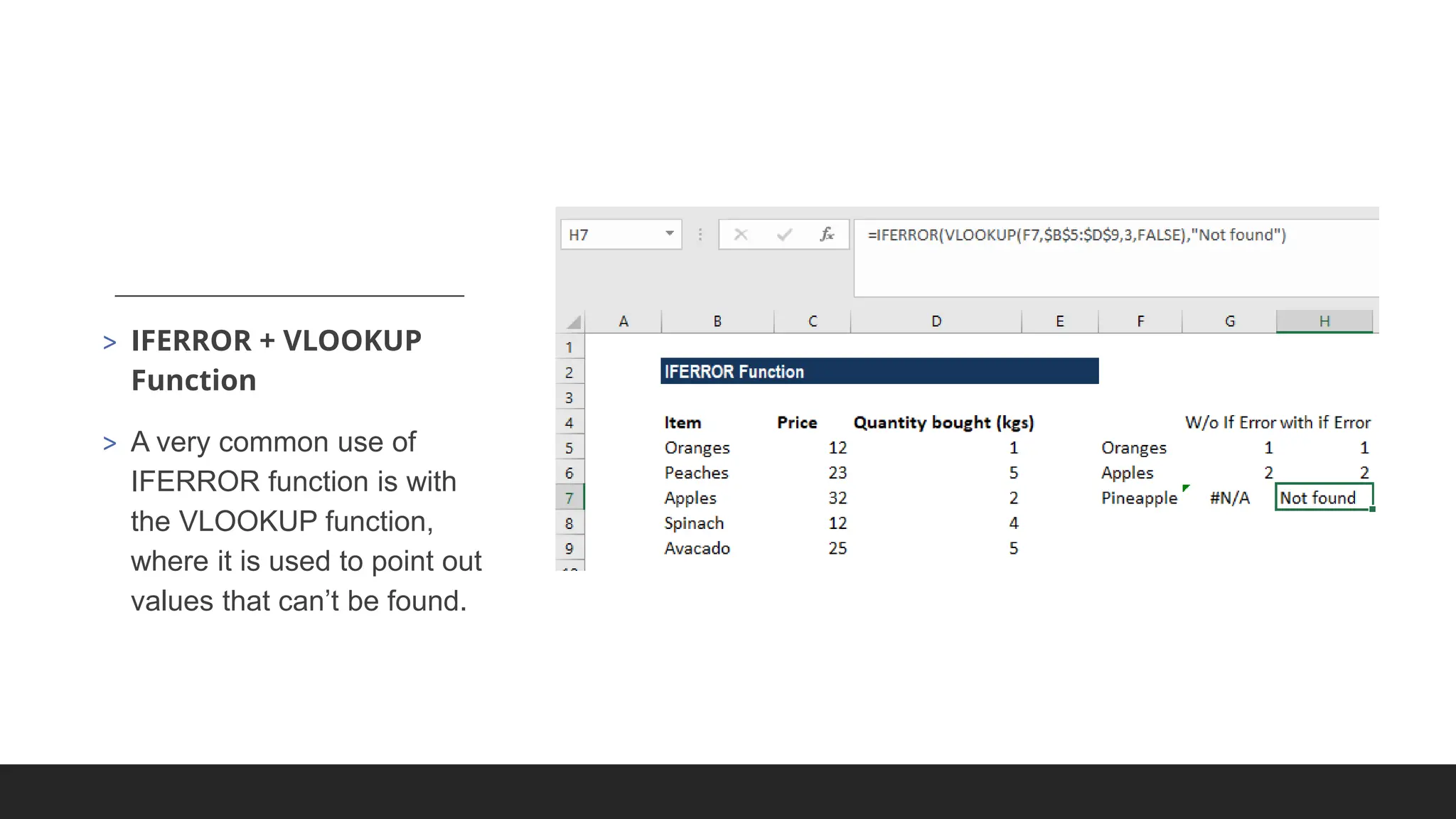
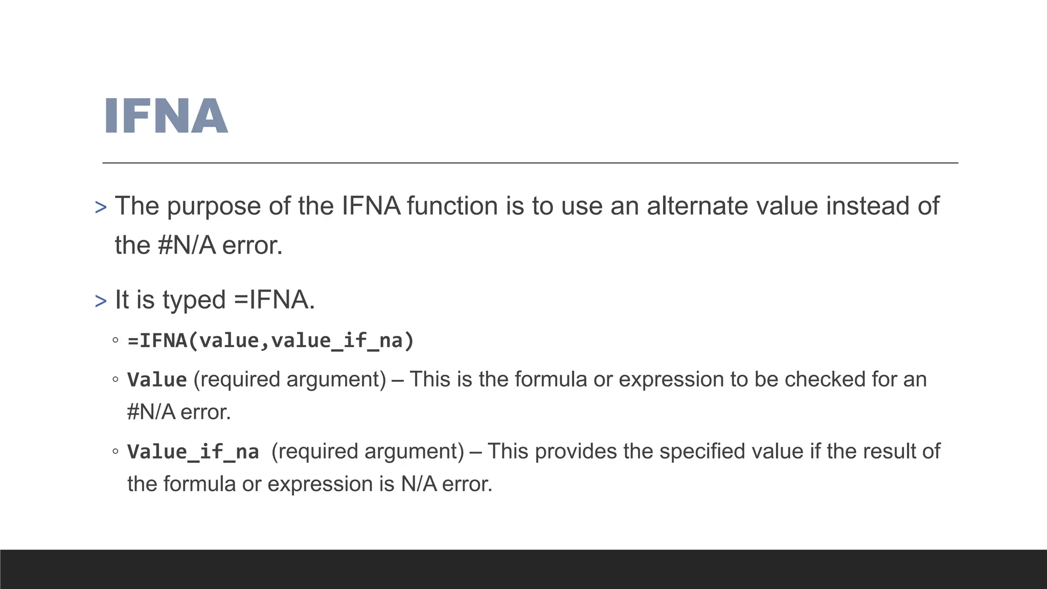
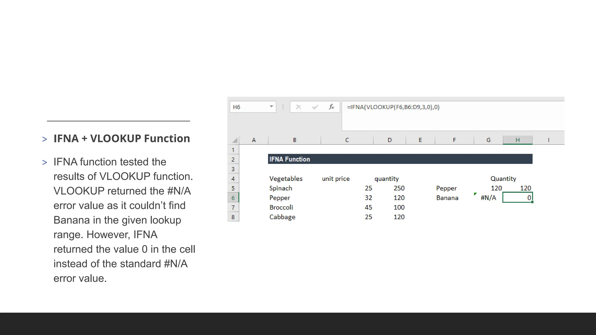
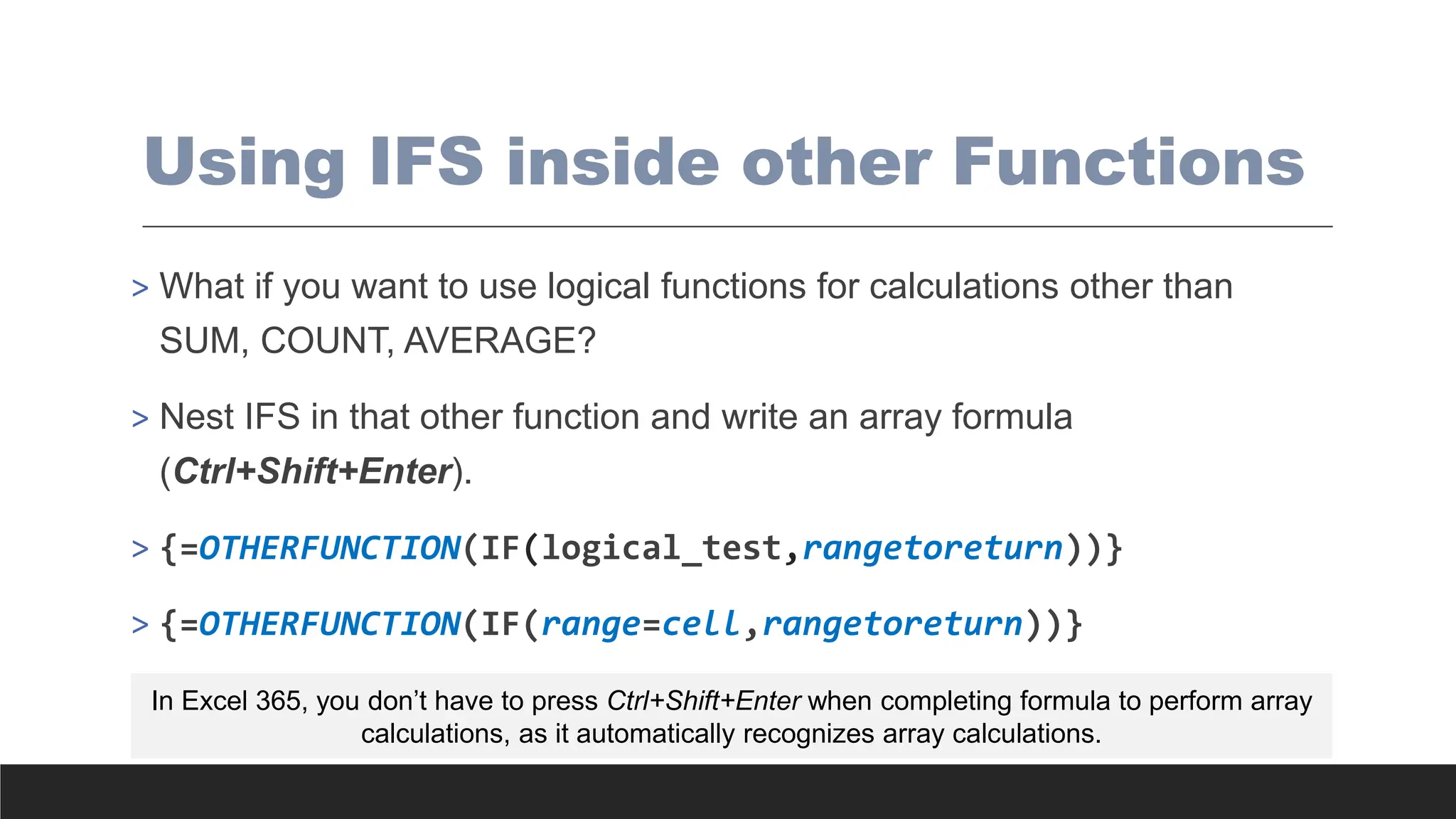
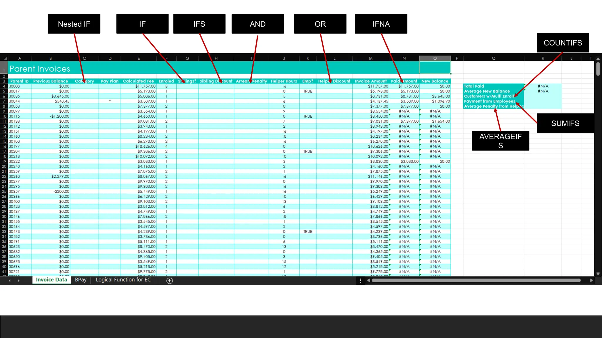
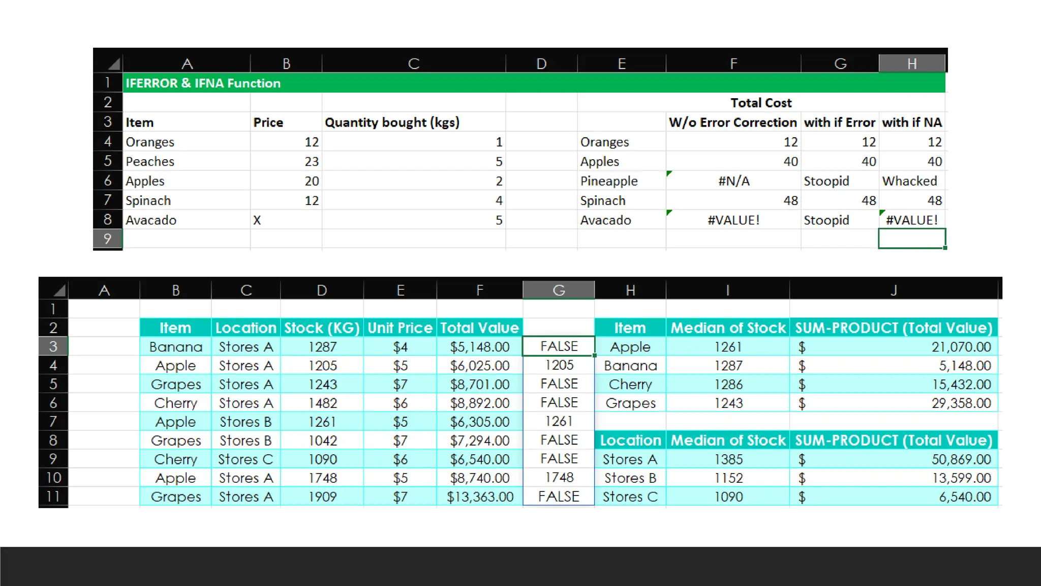

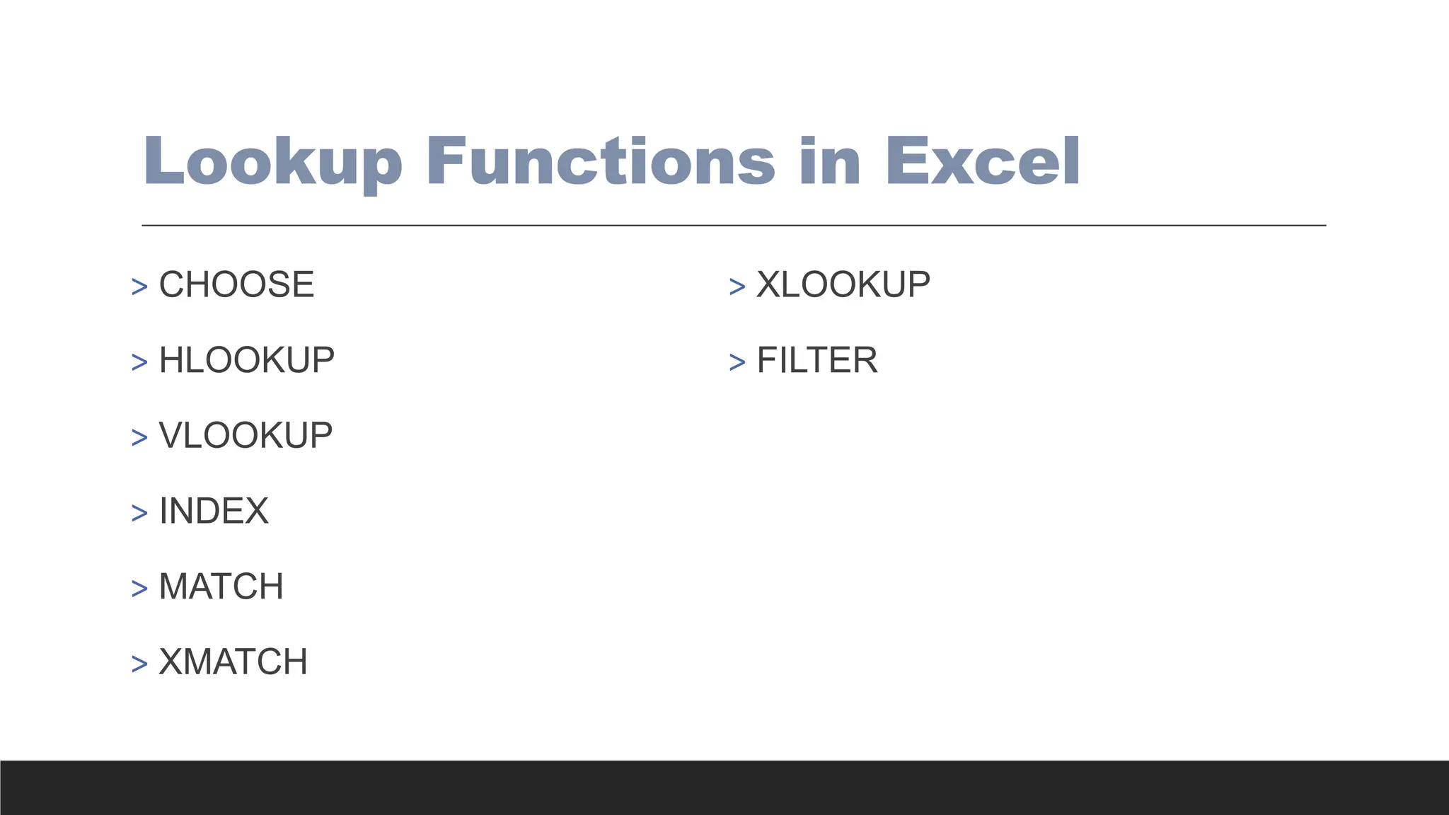
![=CHOOSE(index_num, value1, [value2], ...)
• Index_num - Required. Specifies which value argument is selected. Index_num must
be a number between 1 and 254, or a formula or reference to a cell containing a
number between 1 and 254.
• If index_num is 1, CHOOSE returns value1; if it is 2, CHOOSE returns value2; and so on.
• If index_num is less than 1 or greater than the number of the last value in the list, CHOOSE
returns the #VALUE! error value.
• If index_num is a fraction, it is truncated to the lowest integer before being used.
• Value1, value2, ... - Value 1 is required, subsequent values are optional. 1 to
254 value arguments from which CHOOSE selects a value or an action to perform
based on index_num. The arguments can be numbers, cell references, defined names,
formulas, functions, or text.](https://image.slidesharecdn.com/2-250703033149-22abe271/75/Data-Retrieval-and-Preparation-Business-Analytics-pdf-290-2048.jpg)
![=VLOOKUP (lookup_value, table_array, col_index_num, [range_lookup])
Argument name Description
lookup_value
(required)
The value you want to look up. The value you want to look up must be in
the first column of the range of cells you specify in
the table_array argument.
For example, if table-array spans cells B2:D7, then your lookup_value
must be in column B.
Lookup_value can be a value or a reference to a cell.
table_array (required) The range of cells in which the VLOOKUP will search for
the lookup_value and the return value. You can use a named range or a
table, and you can use names in the argument instead of cell references.
The first column in the cell range must contain the lookup_value. The cell
range also needs to include the return value you want to find.
col_index_num
(required)
The column number (starting with 1 for the left-most column
of table_array) that contains the return value.](https://image.slidesharecdn.com/2-250703033149-22abe271/75/Data-Retrieval-and-Preparation-Business-Analytics-pdf-291-2048.jpg)
![=VLOOKUP (lookup_value, table_array, col_index_num, [range_lookup])
Argument name Description
range_lookup
(optional)
A logical value that specifies whether you want VLOOKUP to find an
approximate or an exact match:
Approximate match - 1/TRUE assumes the first column in the table is
sorted either numerically or alphabetically, and will then search for the
closest value. This is the default method if you don't specify one. For
example, =VLOOKUP(90,A1:B100,2,TRUE).
Exact match - 0/FALSE searches for the exact value in the first column.
For example, =VLOOKUP("Smith",A1:B100,2,FALSE).](https://image.slidesharecdn.com/2-250703033149-22abe271/75/Data-Retrieval-and-Preparation-Business-Analytics-pdf-292-2048.jpg)
![> =INDEX() returns the value of a cell in a table based on the column and row
number.
◦ =INDEX(array, row_num, [column_num])
◦ array - a range of cells that you want to return a value from.
◦ row_num - the row number in array from which you want to return a value. If omitted, the
column_num is required.
◦ column_num - the column number in array from which you want to return a value. If omitted,
row_num is required.](https://image.slidesharecdn.com/2-250703033149-22abe271/75/Data-Retrieval-and-Preparation-Business-Analytics-pdf-293-2048.jpg)
![> =MATCH() & =XMATCH() returns the position of a cell in a row or column.
◦ =MATCH(lookup_value, lookup_array, [match_type])
◦ =XMATCH(lookup_value, lookup_array, [match_mode], [search_mode])
◦ lookup_value – the number or text value you are looking for.
◦ lookup_array – a range of cells being searched.
◦ match_type / match_mode – exact or approximate match modes.
◦ search_mode – order of searching of answer / looking for value.](https://image.slidesharecdn.com/2-250703033149-22abe271/75/Data-Retrieval-and-Preparation-Business-Analytics-pdf-294-2048.jpg)
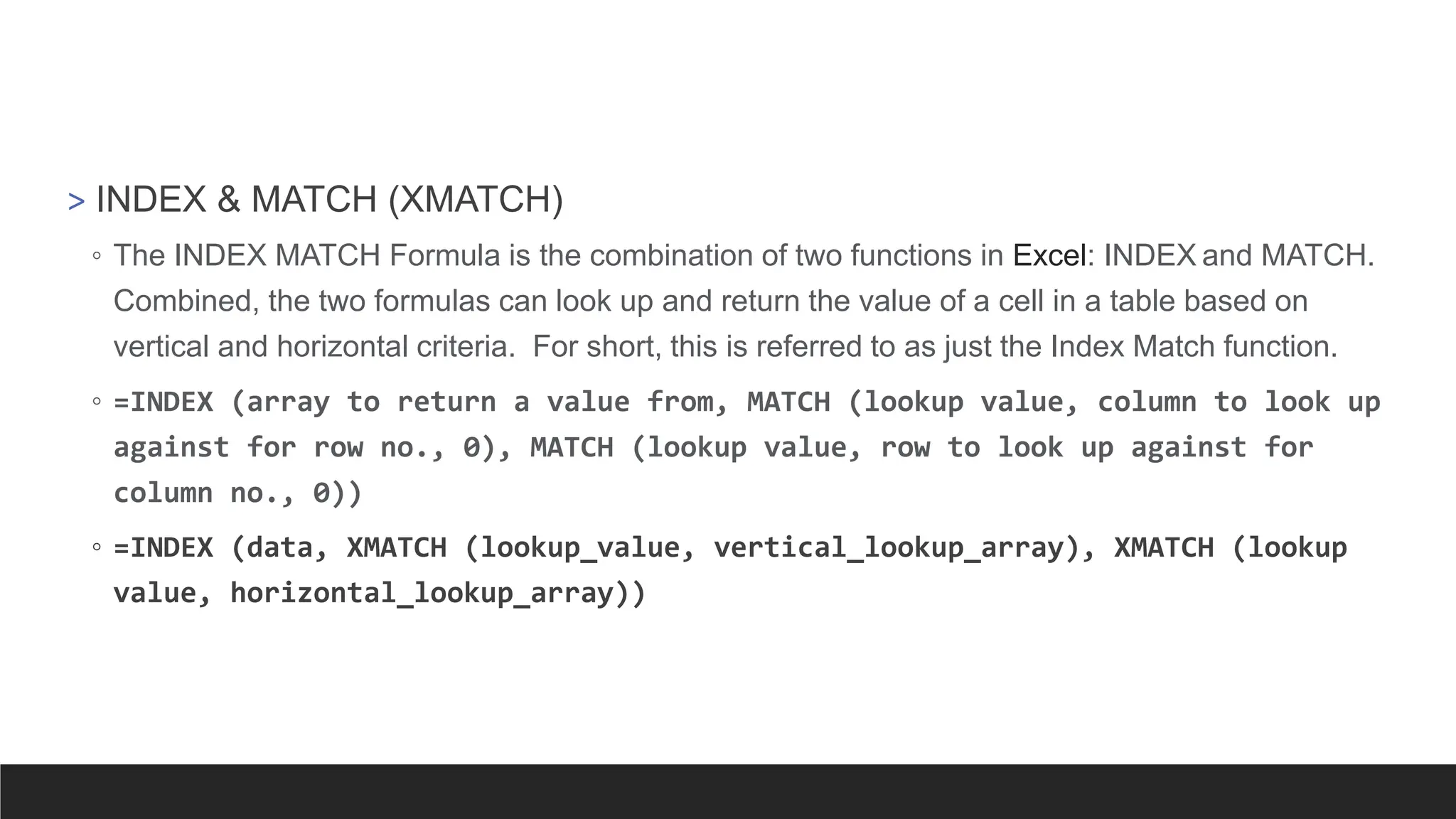
![=XLOOKUP(lookup_value, lookup_array, return_array, [if_not_found],
[match_mode], [search_mode])
Argument Description
lookup_value
Required*
The value to search for
*If omitted, XLOOKUP returns blank cells it finds in lookup_array.
lookup_array
Required
The array or range to search
return_array
Required
The array or range to return](https://image.slidesharecdn.com/2-250703033149-22abe271/75/Data-Retrieval-and-Preparation-Business-Analytics-pdf-296-2048.jpg)
![=XLOOKUP(lookup_value, lookup_array, return_array, [if_not_found],
[match_mode], [search_mode])
Argument Description
[if_not_found]
Optional
Where a valid match is not found, return the [if_not_found] text you supply.
If a valid match is not found, and [if_not_found] is missing, #N/A is returned.
[match_mode]
Optional
Specify the match type:
0 - Exact match. If none found, return #N/A. This is the default.
-1 - Exact match. If none found, return the next smaller item.
1 - Exact match. If none found, return the next larger item.
2 - A wildcard match where *, ?, and ~ have special meaning.
[search_mode]
Optional
Specify the search mode to use:
1 - Perform a search starting at the first item. This is the default.
-1 - Perform a reverse search starting at the last item.
2 - Perform a binary search that relies on lookup_array being sorted
in ascending order. If not sorted, invalid results will be returned.
-2 - Perform a binary search that relies on lookup_array being sorted
in descending order. If not sorted, invalid results will be returned.](https://image.slidesharecdn.com/2-250703033149-22abe271/75/Data-Retrieval-and-Preparation-Business-Analytics-pdf-297-2048.jpg)


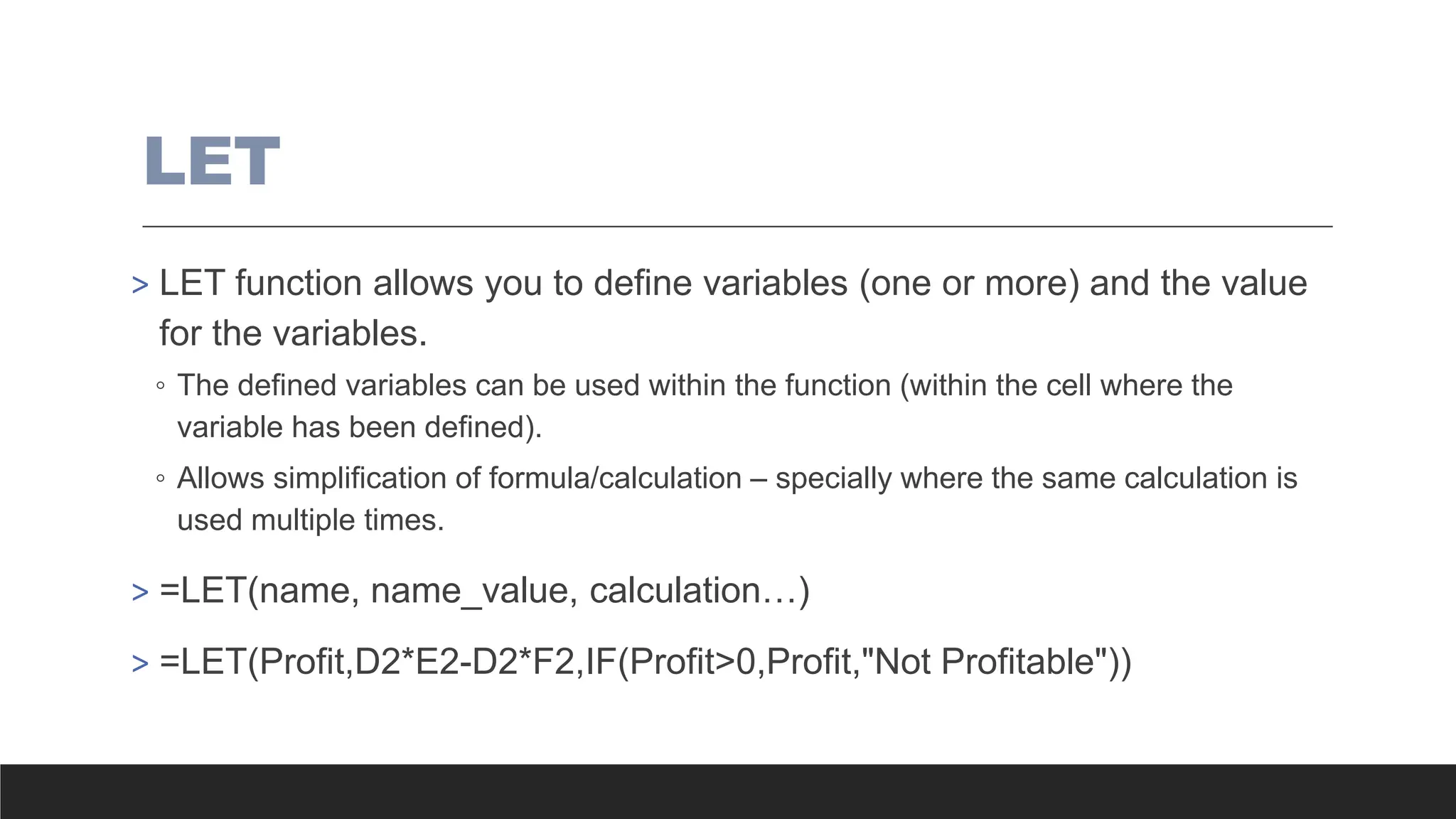
![LAMBDA
> LAMBDA allows you to define a calculation/formula and their inputs.
◦ It essentially names the inputs of a formula and allows you to create a calculation/formula
using the named inputs.
◦ You can then refer to inputs and the inputs will be used to perform the calculation stored in
LAMBDA.
◦ LAMBDA can be combined with named ranges to create a custom function.
> =LAMBDA(parameter or calculation, [parameter or calculation]….)
> =LAMBDA(Volume,Price,Cost, Volume * Price - Volume * Cost)(D2,E2,F2)](https://image.slidesharecdn.com/2-250703033149-22abe271/75/Data-Retrieval-and-Preparation-Business-Analytics-pdf-301-2048.jpg)
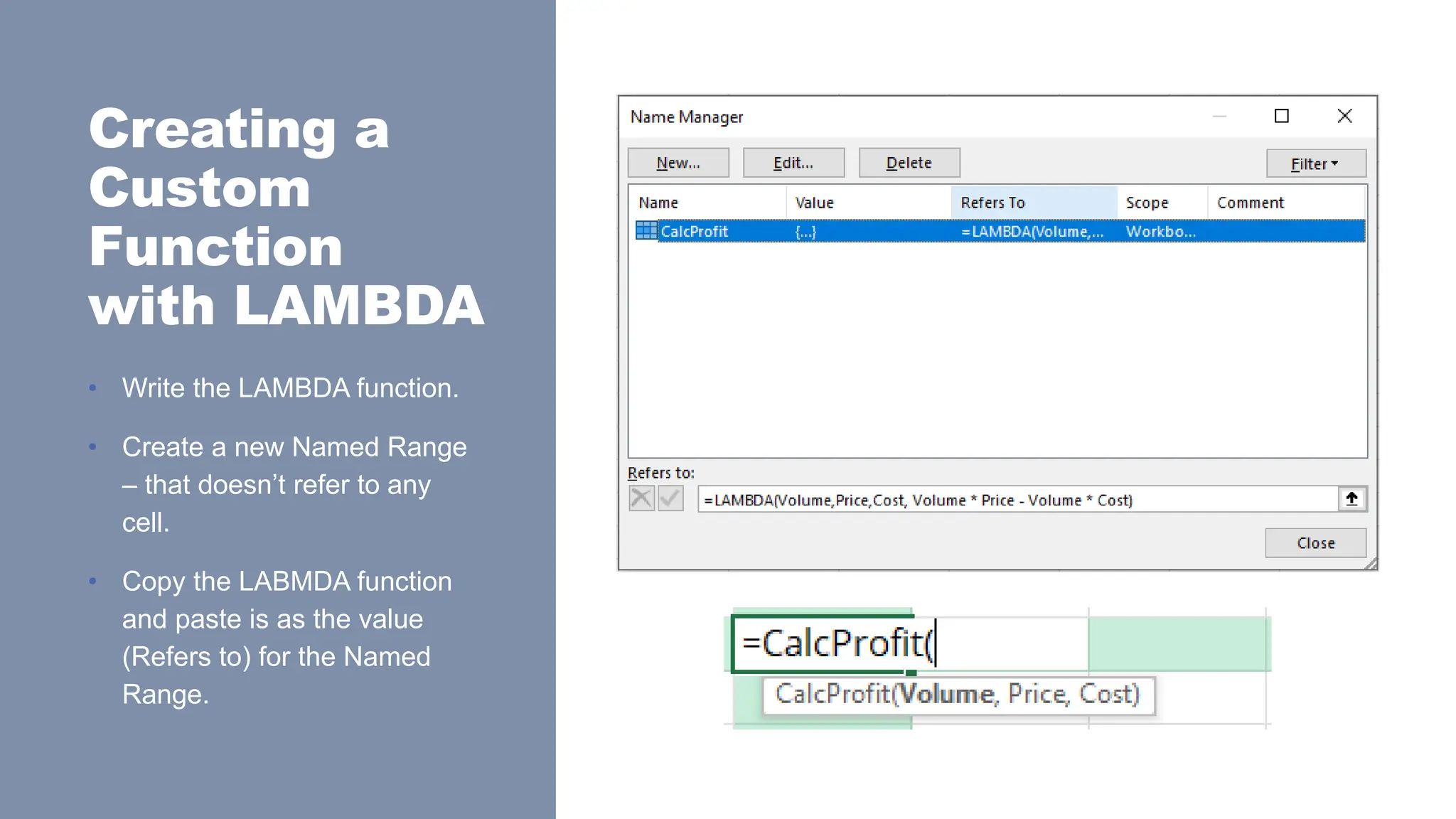


![[DSC Europe 25] Uros Pesic - The Reality of AI in Marketing.pdf](https://cdn.slidesharecdn.com/ss_thumbnails/rtkodnmtycovsllvzsyn-9-251215095918-b0c6bfe3-thumbnail.jpg?width=640&height=640&fit=bounds)


![[DSC Europe 25] Nikolay Burlutskiy - Best Practices for Building Enterprise M...](https://cdn.slidesharecdn.com/ss_thumbnails/uirvaiuvq8y1w8hzd9tx-7-251212103249-2619edb4-thumbnail.jpg?width=640&height=640&fit=bounds)


![[DSC Europe 25] Debmalya Biswas - Agentification: the art of transforming man...](https://cdn.slidesharecdn.com/ss_thumbnails/r5azlggvtqiaiiusrqdr-4-251212103249-5a12c89b-thumbnail.jpg?width=640&height=640&fit=bounds)
![[DSC Europe 25] Dunja Adzic Jovanovic - AI and Cybersecurity: Defending Data ...](https://cdn.slidesharecdn.com/ss_thumbnails/o1zylpbhrtwnixxq2xj8-7-251211083048-185086f6-thumbnail.jpg?width=640&height=640&fit=bounds)
![[DSC Europe 25] Marko Krstic - Understanding the AI Threat Landscape - Risks,...](https://cdn.slidesharecdn.com/ss_thumbnails/tiyim1ins5jvbrvzpzla-2-251209104645-c69d3553-thumbnail.jpg?width=640&height=640&fit=bounds)
![[DSC Europe 25] Milan Sekuloski - Data, Defence, and Development: Cybersecuri...](https://cdn.slidesharecdn.com/ss_thumbnails/dfrkwwx4qly6atqpbl4z-4-251209104645-c3d4b0ca-thumbnail.jpg?width=640&height=640&fit=bounds)
![[DSC Europe 25] Branko Dzakula - From Defense to Attack: How AI Redefines Cyb...](https://cdn.slidesharecdn.com/ss_thumbnails/80bdzdxpr3ky2g0qvyk9-8-251211083048-ce5fc1ee-thumbnail.jpg?width=640&height=640&fit=bounds)
![[DSC Europe 25] Vladimir Jelic - The AI-Driven Security Shift From Reactive D...](https://cdn.slidesharecdn.com/ss_thumbnails/6g5gj25mtjwayniqem1t-6-251209104645-7a5a5fc6-thumbnail.jpg?width=640&height=640&fit=bounds)
![[DSC Europe 25] Dusan Nesic - Securing Tomorrow’s Infrastructure: Why Cyber-P...](https://cdn.slidesharecdn.com/ss_thumbnails/qikbszfftyowjm2q6duw-1-251211083848-8f2ead6b-thumbnail.jpg?width=640&height=640&fit=bounds)
