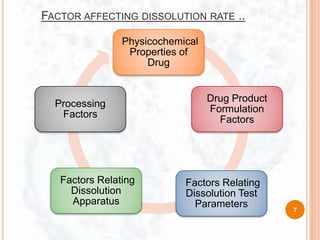
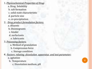
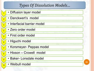
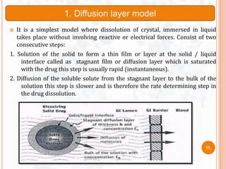
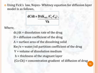
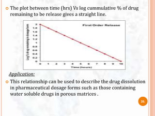
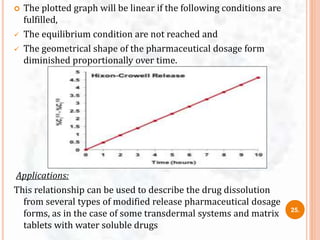
This document provides an outline and introduction to dissolution studies. It discusses what dissolution is, why dissolution studies are important, and factors that can affect dissolution. It also covers different dissolution models, including zero order, first order, Higuchi, and diffusion layer models. The models are used to understand drug release kinetics and develop in vitro-in vivo correlations. Dissolution studies are important tests used to evaluate drug release from dosage forms and ensure batch-to-batch quality and bioavailability.

1. SUBMITTED BY:
Miss. Harshala N. Dhende
First year M.pharm
Sem-I
(Dept. of Pharmaceutics)
DR. D.Y.PATIL COLLEGE OF PHARMACY, AKURDI, PUNE
GUIDED BY:
Prof. Dr. SHILPA P. CHAUDHARI
09/11/2016

2. OUTLINE…….
 Introduction
 What is dissolution
 Why dissolution studies ?
 Factors affecting dissolution
 Dissolution models and its need
 Applications
1

3. INTRODUCTION…
 Drug dissolution is important test used to evaluate drug release of solid and
semisolid dosage forms. This test also quantifies the amount and extent of
drug release from dosage forms.
 The values that are obtained from the dissolution study can be
quantitatively analyzed by using different mathematical formulae, Because
qualitative and quantitative changes in a formulation may alter release of
drug and in vivo performance.s
 Thus mathematical models can be developed. This development requires the
comprehension of all phenomena affecting drug release kinetics and this has
a very important value in the formulation optimization.
 Once a suitable function has been selected, the dissolution profiles are
evaluated depending on the derived model parameters.
2

4. WHAT IS DISSOLUTION?
Dissolution rate may be defined as, “amount of drug
substance that goes in the solution per unit time
under standard conditions of liquid/solid interface,
temperature and solvent composition.”
3

5. THE PROCESSES INVOLVED IN DISSOLUTION OF
TABLET AND CAPSULE:
4fig. 1 different stages depicting the drug absorption
from tablet and capsule.

6. 6
 The release from the tablet is slow. The effectiveness of a
tablet in releasing the drug for absorption depends on two
stages,
a.) initial stage involve breaking of tablet into granules
(disintegration). Sometime , these granules further break
to yeild fine paticle(deaggregation)
b.) the next step involves the releasing of the drug into
solution (dissolution)

7. 1. Results from in-vitro dissolution rate experiments can be used to
explain the observed differences in in-vivo availability.
2. Dissolution testing provides the means to evaluate critical
parameters such as adequate bioavailability and provides
information necessary to formulator in development of more
efficacious and therapeutically optimal dosage forms.
3. Most sensitive and reliable predictors of in-vivo availability.
4. Dissolution analysis of pharmaceutical dosage forms has emerged
as single most important test that will ensure quality of product.
5. It can ensure bioavailability of product between batches that meet
dissolution criteria.
Why dissolution studies?
5

8. 6. Ensure batch-to-batch quality equivalence both in-vitro
and in-vivo, but also to screen formulations during
product development to arrive at optimally effective
products.
7. Physicochemical properties of model can be
understood needed to mimic in-vivo environment.
8. Such models can be used to screen potential drug and
their associated formulations for dissolution and
absorption characteristics.
9. Serve as quality control procedures, once the form of
drug and its formulation have been finalized
6

9. FACTOR AFFECTING DISSOLUTION RATE ..
Physicochemical
Properties of
Drug
Drug Product
Formulation
Factors
Factors Relating
Dissolution Test
Parameters
Factors Relating
Dissolution
Apparatus
Processing
Factors
7

10. 1. Physicochemical Properties of Drug:
a. Drug Solubility
b. salt formation
c. solid state characteristic
d. particle size
e. co-precipitation
2. . Drug product formulation factors:
a. diluents
b. Disintegrants
c. binder
d. surfactants
e. lubricants
3. Processing factors:
a. Method of granulation
b. Compression force
c. Storage condition
4. Factors relating dissolution apparatus and test parameter:
a. agitation
b. Temperature
c. Dissolution medium, pH
8

11.  Dissolution profile:
It is a graphical representation [in term of
concentration vs time ] of complete release of A.P.I. from a
dosage form in an appropriate selected dissolution medium.
i.e. in short it is a measure of release of A.P.I. from dosage
form with respect to time.
IT’s NEED:
 To develop invitro- invivo correlation which can help to
reduce costs, speed up product development.
 To stabilize final dissolution specification for
pharmacological dosage form.
DISSOLUTION MODEL’s AND IT’s NEED
9

12. Types Of Dissolution Models…
1 • Diffusion layer model
2 • Danckwert’s model
3 • Interfacial barrier model
4 • Zero order model
5 • First order model
6 • Higuchi model
7 • Korsmeyer- Peppas model
8 • Hixson – Crowell model
9 • Baker- Lonsdale model
10 • Weibull model
10.

13.  It is a simplest model where dissolution of crystal, immersed in liquid
takes place without involving reactive or electrical forces. Consist of two
consecutive steps:
1. Solution of the solid to form a thin film or layer at the solid / liquid
interface called as stagnant film or diffusion layer which is saturated
with the drug this step is usually rapid (instantaneous).
2. Diffusion of the soluble solute from the stagnant layer to the bulk of the
solution this step is slower and is therefore the rate determining step in
the drug dissolution.
1. Diffusion layer model
11.

14.  Using Fick’s law, Noyes- Whitney equation for diffusion layer
model is as follows,
Where,
dc/dt = dissolution rate of the drug
D = diffusion coefficient of the drug
A = surface area of the dissolving solid
Kw/o = water/oil partition coefficient of the drug
V = volume of dissolution medium
h = thickness of the stagnant layer
(Cs-Cb) = concentration gradient of diffusion of drug
12.

15.  This theory assumes that solid-solution equilibrium is achieved at
interface and mass transport is slow step in dissolution process.
 The model could be visualized as a very thin film having a conc. Ci
which is less than saturation, as it is constantly being exposed to fresh
surfaces of liquid having a conc. much less than Ci.
.
2. Danckwert’s model
13.

16.  Acc. to model, the agitated fluid consist of mass of eddies or packets
that are continuously being exposed to new surfaces of solid and
then carried back to bulk of liquid.
 Diffusion occurs into each of these packets during short time in
which the packet is in contact with surface of solid. Since
turbulence actually extends to surface, there is no laminar
boundary layer and so no stagnant film exists. Instead, surface
continually being replaced with fresh liquid.
The Danckwert’s model can be expressed by the following
equation,
where,
m = mass of solid dissolved
y = rate of surface renewal 14

17.  Interfacial barrier model considers drug dissolution as crystal dissolution
wherein solids get hydrated initially and is not instantaneous.
 In this model it is assumed that the reaction at solid surface is not
instantaneous i.e. the reaction at solid surface and its diffusion across the
interface is slower than diffusion across liquid film.
 therefore the rate of solubility of solid in liquid film becomes the rate
limiting than the diffusion of dissolved molecules .
3. Interfacial Barrier model
15.

18.  When considering the dissolution of crystal will have a
different interfacial barrier given by the following
equation,
where,
Ki = effective interfacial transport constant
dm/dt = Ki (Cs – C)
16

19.  Dissolution of the drug from pharmaceutical dosage forms that do
not disaggregate and release the drug slowly can be represented by
the following equation:
Where,
Wo = the initial amount of drug in the pharmaceutical dosage
form
Wt = the amount of drug in the pharmaceutical dosage form at time t
and K is proportionality constant
The pharmaceutical dosage forms following this profile release the
same amount of drug by unit of time and it is the ideal method of
drug release in order to achieve a pharmacological prolonged
action. The following relation can, in a simple way, express this
model:
4. Zero order model
Wo – Wt = Kt
Qt = Q0 + K0t
17.

20. Where,
Qt = the amount of drug dissolved in time t,
Q0 = the initial amount of drug in the solution and
Ko = the zero order release constant.
To study the release kinetics, data obtained from in vitro drug
release studies were plotted as cumulative amount of drug
released versus time.
• Independent of
concentration
Drug release
rate
• %CDR Vs Tine
• Straight line is obtained
Graphical
representation
18s.

21.  The application of this model to drug dissolution studies was first
proposed by Gibaldi and Feldman (1967) and later by Wagner (1969).
 This model has been also used to describe absorption and/or
elimination of some drugs, although it is difficult to conceptualize this
mechanism in a theoretical basis The dissolution phenomena of a solid
particle in a liquid media imply a surface action, as can be seen by the
Noyes–Whitney Equation:
 Where C is the concentration of the solute in time t, Cs is s order the
solubility in the equilibrium at experience temperature and K is first
order proportionality constant
5. First order model
dc/dt = K (Cs - C)
19.

22.  The plot between time (hrs) Vs log cummulative % of drug
remaining to be release gives a straight line.
Application:
 This relationship can be used to describe the drug dissolution
in pharmaceutical dosage forms such as those containing
water soluble drugs in porous matrices .
20.

23.  This is the first mathematical model that describes drug release
from a matrix system, proposed by Higuchi in 1961 .
 This model is based on different hypothesis that,
 Initial drug concentration in the matrix is much higher than
drug solubility,
 Drug diffusion takes place only in one dimension (Edge effect
should be avoided),
 Drug particles are much smaller than thickness of system,
 swelling of matrix and dissolution are less or negligible,
 Drug diffusivity is constant,
 Perfect sink condition are always attained in the release
environment.
6. Higuchi Model
21.

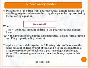
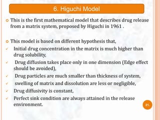
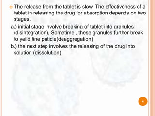
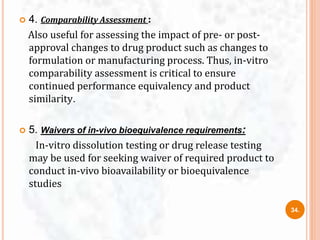
24.  The study of dissolution from a planar system having a
homogeneous matrix can be obtained by the equation:
Where,
A = amount of drug released in time ‘t’ per unit area
D = diffusivity of drug molecule in the matrix substance
C = initial drug concentration
Cs = drug solubility in the matrix media.
A=[D(2C-Cs)Cs X t]1/2
22.

25.  The following graph shows the drug release through
Higuchi Model,
Application :
This relationship can be used to describe the drug
dissolution from several types of modified release
pharmaceutical dosage forms, as in the case of some
transdermal systems and matrix tablets with water soluble
drugs.
23.

26.  Drug powder that having uniformed size particles, Hixson
and Crowell derived the equation which expresses rate of
dissolution based on cube root of weight of particles and
the radius of particle is not assumed to be constant.
This is expressed by the equation,
Where,
Mo = the initial amount of drug in the pharmaceutical
dosage form,
Mt =remaining amount of drug in the pharmaceutical
dosage form at time ‘t’ and κ is proportionality constant
7. Hixson-Crowell Model
Mo1/3 - Mt1/3 = κ t
24.

27.  The plotted graph will be linear if the following conditions are
fulfilled,
 The equilibrium condition are not reached and
 The geometrical shape of the pharmaceutical dosage form
diminished proportionally over time.
Applications:
This relationship can be used to describe the drug dissolution
from several types of modified release pharmaceutical dosage
forms, as in the case of some transdermal systems and matrix
tablets with water soluble drugs
25.

28.  Korsemeyer (1983) derived a simple relationship which described drug
release from a polymeric system equation.
 To find out the mechanism of drug release, first 60% drug release data
were fitted in Korsmeyer -Peppas model.
 The Korsemeyer –Peppas empirical expression relates the function of time
for diffusion controlled mechanism.
 It is given by the equation,
Where,
Mt / M∞ is a fraction of drug released
t = time
k = release rate constant includes structural and geometrical
characteristic of the dosage form
8. Korsemeyer- Peppas model
Mt / M∞ = Ktn
26.

29. n = release component which is indicative of the drug release
mechanism.
where, n is diffusion exponent
i. if n = 1, the release is zero order
ii. if n= 0.5 the release is best described by Fickian diffusion
Application:
This equation has been used to the linearization of release
data from several formulations of microcapsules or microspheres. 27

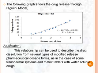
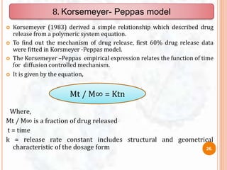
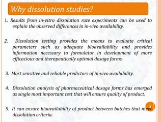
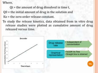
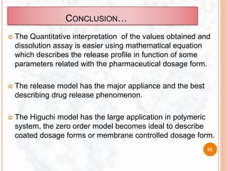
30.  This model was developed by Baker and Lonsdale (1974)
from the Higuchi model and described the drug release from
spherical matrices by using the equation:
Where,
At = drug released amount at time t
A∞ = amount of drug released at an infinite time,
Dm = diffusion coefficient,
Cms = drug solubility in the matrix,
ro = radius of the spherical matrix
Co = initial concentration of drug in the matrix
9. Baker- Lonsdale model
f1= 3/2[1-(1-Ct/C∞)2/3] Ct/C∞ = (3DmCms)/(ro2Co)X t
28.

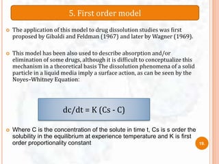
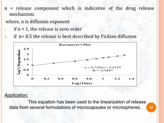
31.  To study the release kinetics, data obtained from in vitro drug
release studies were plotted as [d (At / A∞)] / dt with respect
to the root of time inverse.
Application:
This equation has been used to the linearization of release
data from several formulations of microcapsules or
microspheres.
29.

32.  Wiebull model is generally applied to drug dissolution or release from
pharmaceutical dosage forms
 These accumulated fraction of drug M in solution at time t is given by
Wiebull equation,
Where,
m = % dissolved in time ‘t’
a= scale parameter which defines the time scale of the dissolution
process
Ti = lag time( generally zero)
b = shape factor
What is the need of this equation?
It can be widely used for analysis and characterisation
Of of Drug Dissolution process from different dosage form.
10. Wiebull Model
M= Mo[1-e-(t-T/a)b]
30.

33. HOW TO WE COME TO
KNOW THAT WHICH
MODEL IS FIT?
HOW DO WE
USE THESE
MODELS?
CAN ONE
FORMULATION
FOLLOW DIFFERENT
EQUATION AT A TIME?
 The kinetic model that best fits the dissolution data is evaluated
by comparing the correlation coefficient(r) values obtained in
various models.
The models that gives higher ‘r’ value is the best fit model
Yes, one formulation can follow two type of release system 31.

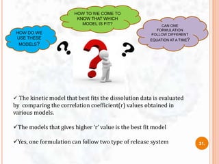
34. Mathematical models for drug release or drug dissolution:
Sr.No. Model Mathematical
equation
Release Mechanism
1 Zero order C=Co-Kot Diffusion Mechanism
2 First order dc/dt = K (CS - C) Fick‟s first law,
diffusion Mechanism
3 Higuchi Model A=[D(2C-Cs)Cs X
t]1/2
Diffusion medium
based Mechanism in
Fick‟s first law
4 Korsemeyer- Peppas
Model
Mt / M∞ = Ktn Peppas Model
Ct/C∞=Ktn Semi empirical
model, diffusion based
mechanism
5 Hixson–Crowell Model Mo1/3 - Mt1/3 = κ t Erosion release
mechanism
6 Weibull Model M= Mo[1-e-(t-T/a)b] Empirical model ,life-
time distribution
function
7 Baker–Lonsdale
Model
f1=3/2[1-(1-
Ct/C∞)2/3] Ct/C∞=Kt
Release of drug from
spherical matrix
32.

35. APPLICATIONS….
 1. Product Development
Important tool during development of dosage form. Aids in guiding the
selection of prototype formulations and for determining optimum
levels of ingredients to achieve drug release profiles, particularly for
extended release formulations. Also guides in selection of a “market-
image” product to be used in pivotal in-vivo bioavailability or
bioequivalence studies.
 2. Quality Assurance:
D.T. performed on future production lots and is used to assess the lot-to-
lot performance characteristics of drug product and provide continued
assurance of product integrity/similarity.
 3. Product Stability:
In-vitro dissolution also used to assess drug product quality with respect
to stability and shelf- life. As product age, physicochemical changes to
the dosage form may alter dissolution characteristics of drug product
over time. For some products, polymorph transformations to more
stable, and hence less soluble crystalline forms may result in reduced
dissolution rates. .
33.

36.  4. Comparability Assessment :
Also useful for assessing the impact of pre- or post-
approval changes to drug product such as changes to
formulation or manufacturing process. Thus, in-vitro
comparability assessment is critical to ensure
continued performance equivalency and product
similarity.
 5. Waivers of in-vivo bioequivalence requirements:
In-vitro dissolution testing or drug release testing
may be used for seeking waiver of required product to
conduct in-vivo bioavailability or bioequivalence
studies
34.

37. CONCLUSION…
 The Quantitative interpretation of the values obtained and
dissolution assay is easier using mathematical equation
which describes the release profile in function of some
parameters related with the pharmaceutical dosage form.
 The release model has the major appliance and the best
describing drug release phenomenon.
 The Higuchi model has the large application in polymeric
system, the zero order model becomes ideal to describe
coated dosage forms or membrane controlled dosage form.
35.

38. REFERENCES:
1.) Mathematical Models of Drug Dissolution: A Review, Ramteke K.H.
Dighe P.A.Kharat A. R. Patil S.V. ,
PES’s Modern College of Pharmacy (for ladies), Moshi, Pune, India .
Ashokrao Mane College of Pharmacy, Peth-Vadgaon, Kolhapur, India.
2.) Remington’s “ The science and practice of pharmacy”,
21st edition, page no. 672-685
3) Leon Shargel, Andrew, “A textbook of applied Bio pharmaceutics and
Pharmacokinetics”, 4th edition, page no. 131-195
4) Brahmankar, “A textbook of Bio pharmaceutics and Pharmacokinetic”,
3rd edition, page no.15-48.
5) C.V.S. Subrahmanyam, ”Textbook of Physical Pharmaceutics”, 2nd
edition, Vallabh Prakashan, page no. 85-109
36.

39. 38.