Downloaded 28 times


![Abstraction of Pressure Transmission (1)
[Model 1]
[Model 2] [Model 3]
63](https://image.slidesharecdn.com/dissertationslides-1328181828655-phpapp01-120202052733-phpapp01/85/Dissertation-Slides-63-320.jpg)


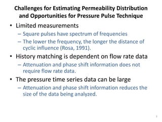
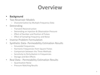
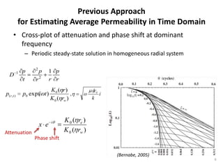
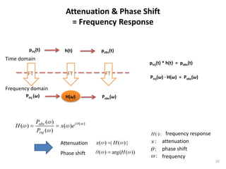
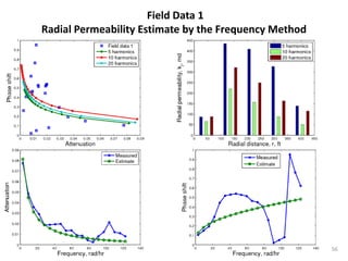
The document discusses using pressure pulse testing to characterize heterogeneous reservoirs. It investigates how frequency response represents heterogeneity and formulates periodic steady-state solutions for radial and vertical permeability distributions. The overall procedure is to apply pressure pulses at multiple frequencies, analyze the attenuation and phase shift response, and determine the permeability distribution by solving the inverse problem. The goal is to provide a new method for characterizing heterogeneous reservoirs using frequency-domain analysis of pressure pulse test data.