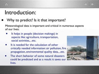
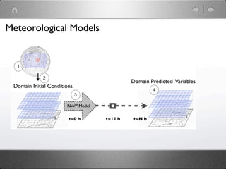
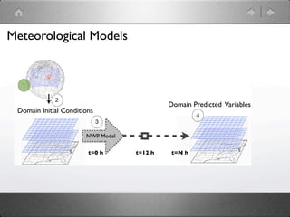
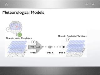
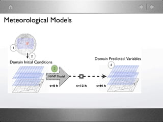
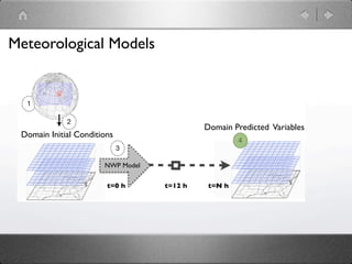
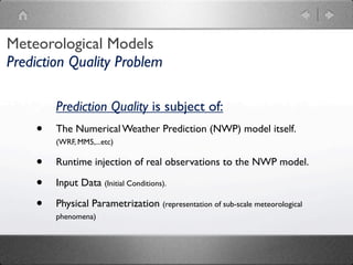
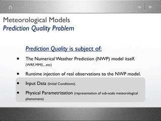
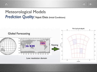
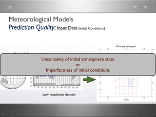
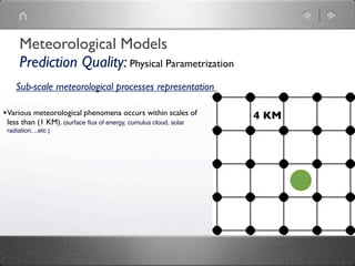
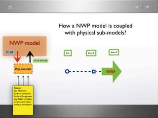
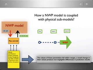
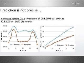
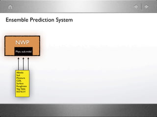
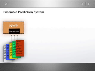
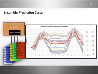
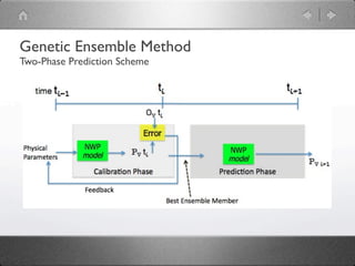
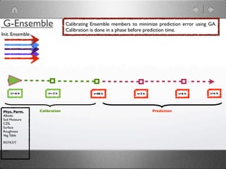
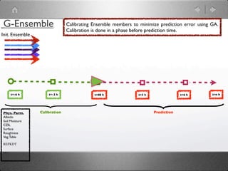
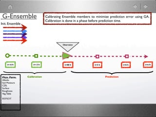
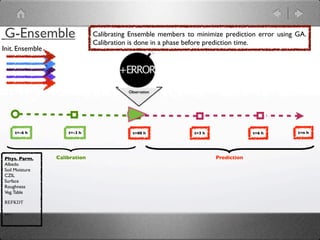
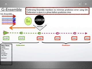
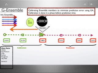
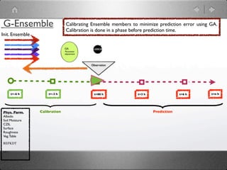
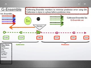
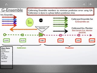
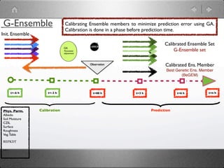
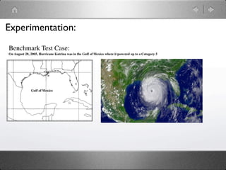
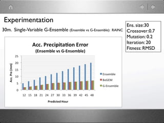
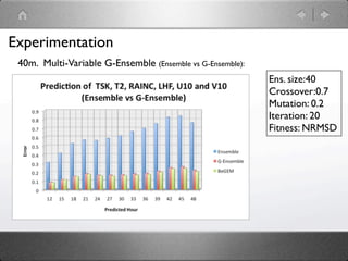
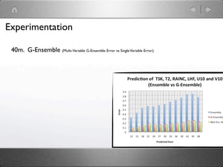
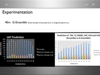
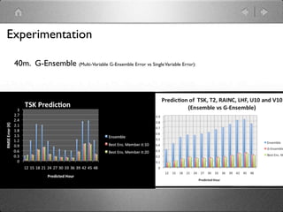
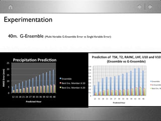
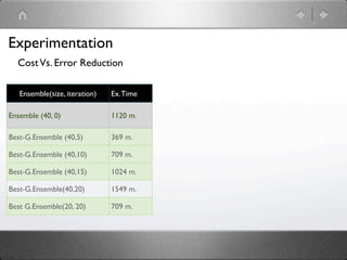
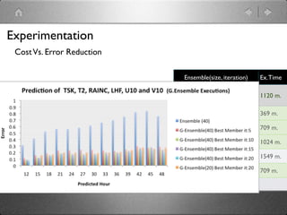
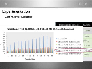
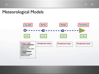
Genetic Ensemble (G-Ensemble) for
   Meteorological Prediction
          Enhancement
                 Hisham Ihshaish, Ana Cortés, and Miquel A. Senar

                  hisham@caos.uab.es, {ana.cortes,miquelangel.senar}@uab.es

  Computer Architecture &
Operating Systems Department
                                      Barcelona, Spain

   The 2011 International Conference on Parallel and Distributed Processing Techniques and
                                  Applications (PDPTA´11)
                                        18-21, July, 2011
                                    Las Vegas, Nevada, USA
Presentation:
 •   Introduction.

 •   Meteorological Models.

 •   Problem and Methodology.

 •   Experimentation.

 •   Conclusions and Future Work.
Introduction:
Introduction:
•   Why to predict? Is it that important?
Introduction:
•    Why to predict? Is it that important?
    Meteorological data is important and critical in numerous aspects
    of our lives:
Introduction:
•       Why to predict? Is it that important?
    Meteorological data is important and critical in numerous aspects
    of our lives:
    •     It helps in people (decision makings) in
          aspects like: agriculture, transportation,
          social activities,...etc.
    •    It is needed for the calculation of other
         critically needed information: air pollution, fire
         propagation, environmental quality data,...etc.
    •   The short behavior of some natural disasters
        could be predicted and as a result: it saves our
        lives.
Meteorological Models


  1

             2
                                            Domain Predicted Variables
 Domain Initial Conditions
                                                     4
                             3

                       NWP Model

                        t=0 h      t=12 h    t=N h
Meteorological Models
      * Dt = 90 km


  1

                 2
      Level 3                               Domain Predicted Variables
 Domain Initial Conditions
                                                     4
                             3

      Level 2          NWP Model

                        t=0 h      t=12 h    t=N h

       Level 1
Meteorological Models


  1

             2
                                            Domain Predicted Variables
 Domain Initial Conditions
                                                     4
                             3

                       NWP Model

                        t=0 h      t=12 h    t=N h
Meteorological Models
Prediction Quality Problem

        Prediction Quality is subject of:
    •   The Numerical Weather Prediction (NWP) model itself.
        (WRF, MM5,...etc)

    •   Runtime injection of real observations to the NWP model.

    •   Input Data (Initial Conditions).

    •   Physical Parametrization (representation of sub-scale meteorological
        phenomena)
Meteorological Models
Prediction Quality: Input Data (Initial Conditions)
Meteorological Models
Prediction Quality: Input Data (Initial Conditions)


  Global Forecasting


                36 KM


                 Low resolution domain
Meteorological Models
Prediction Quality: Input Data (Initial Conditions)


  Global Forecasting


                               4 KM
                36 KM


                 Low resolution domain
Meteorological Models
Prediction Quality: Input Data (Initial Conditions)


  Global Forecasting


                               4 KM
                                         Nesting
                36 KM


                 Low resolution domain
Meteorological Models
Prediction Quality: Input Data (Initial Conditions)


  Global Forecasting


                               4 KM
                                         Nesting
                36 KM


                 Low resolution domain
Meteorological Models
Prediction Quality: Input Data (Initial Conditions)


  Global Forecasting
                Uncertainty of initial atmosphere state
                                   or
                   Imperfectness of initial conditions
                            4 KM
                                        Nesting
                36 KM


                 Low resolution domain
Meteorological Models
Prediction Quality: Physical Parametrization
Sub-scale meteorological processes representation
Meteorological Models
      Prediction Quality: Physical Parametrization
    Sub-scale meteorological processes representation

• Various meteorological phenomena occurs within scales of        4 KM
 less than (1 KM). (surface flux of energy, cumulus cloud, solar
 radiation, ..etc )
Meteorological Models
      Prediction Quality: Physical Parametrization
    Sub-scale meteorological processes representation

• Various meteorological phenomena occurs within scales of        4 KM
 less than (1 KM). (surface flux of energy, cumulus cloud, solar
 radiation, ..etc )

• To represent this process in domain scale, NWP model is
 coupled with physical sub-models that includes these
 processes in domain grid points.

• Physical sub-models provide NWP models with a set of
 variables by calculating high-resolution data that
 characterize each sub-scale phenomena or process.
How a NWP model is coupled
              with physical sub-models?
NWP model
              t=x     t=x+1


                      WRF
How a NWP model is coupled
                                                    with physical sub-models?
  NWP model
ST, HF                                              t=x     t=x+1


                                ST, HF, SM, DSE


          Phys. sub.mdel
                                                            WRF


         Albedo
         Soil Moisture
         Surface emissivity
         Surface Roughness
         Veg. Table variables
         Evaporation ratios
         Surface absorption
         .
         .
How a NWP model is coupled
                                                    with physical sub-models?
  NWP model
ST, HF                                              t=x     t=x+1    t=x+2


                                ST, HF, SM, DSE


          Phys. sub.mdel
                                                                    WRF


         Albedo
         Soil Moisture
         Surface emissivity
         Surface Roughness
         Veg. Table variables
         Evaporation ratios
         Surface absorption
         .
         .
How a NWP model is coupled
                                                    with physical sub-models?
  NWP model
ST, HF                                               t=x              t=x+1            t=x+2


                                ST, HF, SM, DSE


          Phys. sub.mdel
                                                                                    WRF


         Albedo
         Soil Moisture
         Surface emissivity
         Surface Roughness
                                                   The values of these parameters fall within ranges, a small change in
         Veg. Table variables
         Evaporation ratios                        their values produce non-negligible differences in prediction results
         Surface absorption
         .
         .
Prediction is not precise....

Hurricane Katrina Case: Prediction of 28.8.2005 at 12:00h. to
30.8.2005 at 24:00 (36 hours):
           400.00                                                                    40


                                                            Acc . Precipitation mm
           325.00                                                                    33
LHF W/m2


           250.00                                                                    26


           175.00                                                                    19

                         Observed          Predicted                                                Observed        Predicted
           100.00                                                                    12
                    12     21         30          39   48                                 12   21     30       39         48
                                    H o u r                                                         H o u r
NWP Enhancement
Ensemble Prediction System (EPS)

•   The Basic idea of an EPS method is to reflect the possible
    variations in initial conditions and physical parameters in the
    final result of the meteorological prediction.

•   A set of predictions is conducted, each of which considers a
    different combination of initial conditions or physical
    parameters.

•   The average of all predictions´ results is considered as the
    final result of prediction
Ensemble Prediction System


   NWP
   Phys. sub.mdel


    Albedo
    Soil
    Moisture
    CZIL
    Surface
    Roughness
    Veg. Table
    REFKDT
Ensemble Prediction System


        NWP
        Phys. sub.mdel


                      Albedo
                AlbedoSoil
           Albedo
                Soil Moisture
     AlbedoSoil Moisture
Albedo Moisture CZIL
     Soil       CZIL Surface
Soil Moisture Surface
           CZIL
Moisture Surface
     CZIL             Roughness
                Roughness
CZIL       Roughness Veg. Table
     Surface    Veg. Table
Surface Veg. Table REFKDT
     Roughness REFKDT
Roughness
     Veg. Table
           REFKDT
Veg. Table
     REFKDT
REFKDT
Ensemble Prediction System


        NWP
           Ensemble Prediction costs (computationally) and
        Phys. sub.mdel

                       normally not precise!

                Albedo
           Albedo
                      Albedo
                      Soil
                Soil Moisture
                                  What do we propose?
     AlbedoSoil Moisture
Albedo Moisture CZIL
     Soil       CZIL Surface
Soil Moisture Surface
           CZIL
Moisture Surface
     CZIL             Roughness
                Roughness
CZIL       Roughness Veg. Table
     Surface    Veg. Table
Surface Veg. Table REFKDT
     Roughness REFKDT
Roughness
     Veg. Table
           REFKDT
Veg. Table
     REFKDT
REFKDT
Genetic Ensemble Method
Two-Phase Prediction Scheme
G-Ensemble
G-Ensemble                     Calibrating Ensemble members to minimize prediction error using GA.
                               Calibration is done in a phase before prediction time.
Init. Ensemble


      t=-6 h         t=-3 h                t=00 h             t=3 h                t=6 h       t=n h


Phys. Parm.      Calibration                                          Prediction
Albedo
Soil Moisture
CZIL
Surface
Roughness
Veg. Table

REFKDT

...
G-Ensemble                     Calibrating Ensemble members to minimize prediction error using GA.
                               Calibration is done in a phase before prediction time.
Init. Ensemble


                                          Observation


      t=-6 h         t=-3 h                 t=00 h            t=3 h                t=6 h       t=n h


Phys. Parm.      Calibration                                          Prediction
Albedo
Soil Moisture
CZIL
Surface
Roughness
Veg. Table

REFKDT

...
G-Ensemble                     Calibrating Ensemble members to minimize prediction error using GA.
                               Calibration is done in a phase before prediction time.
Init. Ensemble

                               GA
                               Parameter
                               adjustment


                                            Observation


      t=-6 h         t=-3 h                   t=00 h          t=3 h                t=6 h       t=n h


Phys. Parm.      Calibration                                          Prediction
Albedo
Soil Moisture
CZIL
Surface
Roughness
Veg. Table

REFKDT

...
G-Ensemble                     Calibrating Ensemble members to minimize prediction error using GA.
                               Calibration is done in a phase before prediction time.
Init. Ensemble
                                                                             Calibrated Ensemble Set
                               GA
                               Parameter                                         G-Ensemble set
                               adjustment


                                            Observation


      t=-6 h         t=-3 h                   t=00 h          t=3 h                t=6 h         t=n h


Phys. Parm.      Calibration                                          Prediction
Albedo
Soil Moisture
CZIL
Surface
Roughness
Veg. Table

REFKDT

...
G-Ensemble                     Calibrating Ensemble members to minimize prediction error using GA.
                               Calibration is done in a phase before prediction time.
Init. Ensemble
                                                                             Calibrated Ensemble Set
                               GA
                               Parameter                                         G-Ensemble set
                               adjustment


                                            Observation                      Calibrated Ens. Member
                                                                              Best Genetic Ens. Member
                                                                                      (BeGEM)


      t=-6 h         t=-3 h                   t=00 h          t=3 h                t=6 h           t=n h


Phys. Parm.      Calibration                                          Prediction
Albedo
Soil Moisture
CZIL
Surface
Roughness
Veg. Table

REFKDT

...
G-Ensemble Calibration Error
Depending on the error function used, two G-Ensemble strategies are presented:
 1) Single-Variable G-Ensemble

  Fitness =

  Fitness for wind component = 7.3 m/s                  Fitness for temperature = 4.2 c or k
G-Ensemble Calibration Error
Depending on the error function used, two G-Ensemble strategies are presented:
 1) Single-Variable G-Ensemble

  Fitness =

  Fitness for wind component = 7.3 m/s                  Fitness for temperature = 4.2 c or k


 2) Multi-Variable G-Ensemble
We use a Normalized RMSD in order to be able to enhance predictions of a set of meteorological
variables together.

The normalized root mean squared deviation or error (NRMSD or NRMSE) is the
RMSD divided by the range of observed values:


   Fitness for wind component = 9.1%                   Fitness for temperature = 3.7%

         Fitness (of all) = NRMSD(wind)+ NRMSD(T)+ NRMSD(RAINC) = value%
Experimentation:
Benchmark Test Case:
On August 28, 2005, Hurricane Katrina was in the Gulf of Mexico where it powered up to a Category 5


              Gulf of Mexico
Experimentation
Experimentation
Temperature 2m:           T2              Sea Surface Temperature:           TSK


Latent Heat Flux:         LHF             Wind component: velocity in east-west direction
                                                                V10


Wind component: velocity in north-south   Accumulated Precipitation:RAINC
               direction U10


1. Prediction is held 28.8.2005 at 12:00h. to 30.8.2005 at 24:00 (36 hours)
2. Initializing Ensemble combinations of different input data variables randomly.
3. Applying GA to calibrate input variables of LSM sub-model to generate
Genetic Ensembles
Experimentation
30m. Single-Variable G-Ensemble (Ensemble vs G-Ensemble): LHF   Ens. size:30
                                                                Crossover:0.7
                                                                Mutation: 0.2
                                                                Iteration: 20
                                                                Fitness: RMSD
Experimentation
                                                                    Ens. size:30
30m. Single-Variable G-Ensemble (Ensemble vs G-Ensemble):   RAINC   Crossover:0.7
                                                                    Mutation: 0.2
                                                                    Iteration: 20
                                                                    Fitness: RMSD
Experimentation
 40m. Multi-Variable G-Ensemble (Ensemble vs G-Ensemble):
                                                            Ens. size:40
                                                            Crossover:0.7
                                                            Mutation: 0.2
                                                            Iteration: 20
                                                            Fitness: NRMSD
Experimentation

 40m. G-Ensemble (Multi-Variable G-Ensemble Error vs Single Variable Error):
Experimentation

 40m. G-Ensemble (Multi-Variable G-Ensemble Error vs Single Variable Error):
Experimentation

 40m. G-Ensemble (Multi-Variable G-Ensemble Error vs Single Variable Error):
Experimentation

 40m. G-Ensemble (Multi-Variable G-Ensemble Error vs Single Variable Error):
Experimentation
  Cost Vs. Error Reduction

   Ensemble(size, iteration)   Ex. Time

Ensemble (40, 0)               1120 m.

Best-G.Ensemble (40,5)         369 m.

Best-G.Ensemble (40,10)        709 m.

Best-G.Ensemble (40,15)        1024 m.

Best-G.Ensemble(40,20)         1549 m.

Best G.Ensemble(20, 20)        709 m.
Experimentation
 Cost Vs. Error Reduction

                               Ensemble(size, iteration)   Ex. Time

                            Ensemble (40, 0)               1120 m.

                            Best-G.Ensemble (40,5)         369 m.

                            Best-G.Ensemble (40,10)        709 m.

                            Best-G.Ensemble (40,15)        1024 m.

                            Best-G.Ensemble(40,20)         1549 m.

                            Best G.Ensemble(20, 20)        709 m.
Conclusions and Future Work
 •   We proposed a methodology to enhance methodological prediction process,
     using Genetic Algorithm functions and techniques.

 •   Our method depends on the adjustment of input data set that causes less
     possible error compared with observations.

 •   We did also experiments on more cases and predictions are enhanced using
     our method. and we will make more experiments to cover real prediction cases.

 •   In scenarios with a limited number of computing resources, in which EPS could
     not be used due to its time constraints, G-Ensemble stands to be a good
     alternative choice.

 •   Thanks to the enhancement in prediction accuracy, more sophisticated schemes
     might be developed in the near future by injecting observed meteorological variables
     at run-time.
Genetic Ensemble (G-Ensemble) for
   Meteorological Prediction
          Enhancement

  Hisham Ihshaish, Ana Cortés, and Miquel A. Senar

   hisham@caos.uab.es, {ana.cortes,miquelangel.senar}@uab.es


                        Thanks!

                     Questions?
Meteorological Models


   •   The aim of a meteorological model is to predict
       the atmospheric state in the future:
Meteorological Models

                Now 00:00                Mid Day           Midnight         Tom.Mid Day


                 t=0 h                    t=12 h            t=24 h             t=36 h


         Initial state                Predicted state   Predicted state   Predicted state
         1. surface properties:
         elevation, land use,
         vegetation index,
         temperature of sea surface
         temperature, ...
         2. meteorological
         variables:
         temperature, humidity,
         pressure and wind

Pdpta11 G-Ensemble for Meteorological Prediction Enhancement

  • 1.
    Genetic Ensemble (G-Ensemble)for Meteorological Prediction Enhancement Hisham Ihshaish, Ana Cortés, and Miquel A. Senar hisham@caos.uab.es, {ana.cortes,miquelangel.senar}@uab.es Computer Architecture & Operating Systems Department Barcelona, Spain The 2011 International Conference on Parallel and Distributed Processing Techniques and Applications (PDPTA´11) 18-21, July, 2011 Las Vegas, Nevada, USA
  • 2.
    Presentation: • Introduction. • Meteorological Models. • Problem and Methodology. • Experimentation. • Conclusions and Future Work.
  • 3.
  • 4.
    Introduction: • Why to predict? Is it that important?
  • 5.
    Introduction: • Why to predict? Is it that important? Meteorological data is important and critical in numerous aspects of our lives:
  • 6.
    Introduction: • Why to predict? Is it that important? Meteorological data is important and critical in numerous aspects of our lives: • It helps in people (decision makings) in aspects like: agriculture, transportation, social activities,...etc. • It is needed for the calculation of other critically needed information: air pollution, fire propagation, environmental quality data,...etc. • The short behavior of some natural disasters could be predicted and as a result: it saves our lives.
  • 7.
    Meteorological Models 1 2 Domain Predicted Variables Domain Initial Conditions 4 3 NWP Model t=0 h t=12 h t=N h
  • 8.
    Meteorological Models 1 2 Domain Predicted Variables Domain Initial Conditions 4 3 NWP Model t=0 h t=12 h t=N h
  • 9.
    Meteorological Models 1 2 Domain Predicted Variables Domain Initial Conditions 4 3 NWP Model t=0 h t=12 h t=N h
  • 10.
    Meteorological Models * Dt = 90 km 1 2 Level 3 Domain Predicted Variables Domain Initial Conditions 4 3 Level 2 NWP Model t=0 h t=12 h t=N h Level 1
  • 11.
    Meteorological Models 1 2 Domain Predicted Variables Domain Initial Conditions 4 3 NWP Model t=0 h t=12 h t=N h
  • 12.
    Meteorological Models 1 2 Domain Predicted Variables Domain Initial Conditions 4 3 NWP Model t=0 h t=12 h t=N h
  • 13.
    Meteorological Models 1 2 Domain Predicted Variables Domain Initial Conditions 4 3 NWP Model t=0 h t=12 h t=N h
  • 14.
    Meteorological Models Prediction QualityProblem Prediction Quality is subject of: • The Numerical Weather Prediction (NWP) model itself. (WRF, MM5,...etc) • Runtime injection of real observations to the NWP model. • Input Data (Initial Conditions). • Physical Parametrization (representation of sub-scale meteorological phenomena)
  • 15.
    Meteorological Models Prediction QualityProblem Prediction Quality is subject of: • The Numerical Weather Prediction (NWP) model itself. (WRF, MM5,...etc) • Runtime injection of real observations to the NWP model. • Input Data (Initial Conditions). • Physical Parametrization (representation of sub-scale meteorological phenomena)
  • 16.
    Meteorological Models Prediction Quality:Input Data (Initial Conditions)
  • 17.
    Meteorological Models Prediction Quality:Input Data (Initial Conditions) Global Forecasting 36 KM Low resolution domain
  • 18.
    Meteorological Models Prediction Quality:Input Data (Initial Conditions) Global Forecasting 4 KM 36 KM Low resolution domain
  • 19.
    Meteorological Models Prediction Quality:Input Data (Initial Conditions) Global Forecasting 4 KM Nesting 36 KM Low resolution domain
  • 20.
    Meteorological Models Prediction Quality:Input Data (Initial Conditions) Global Forecasting 4 KM Nesting 36 KM Low resolution domain
  • 21.
    Meteorological Models Prediction Quality:Input Data (Initial Conditions) Global Forecasting Uncertainty of initial atmosphere state or Imperfectness of initial conditions 4 KM Nesting 36 KM Low resolution domain
  • 22.
    Meteorological Models Prediction Quality:Physical Parametrization Sub-scale meteorological processes representation
  • 23.
    Meteorological Models Prediction Quality: Physical Parametrization Sub-scale meteorological processes representation • Various meteorological phenomena occurs within scales of 4 KM less than (1 KM). (surface flux of energy, cumulus cloud, solar radiation, ..etc )
  • 24.
    Meteorological Models Prediction Quality: Physical Parametrization Sub-scale meteorological processes representation • Various meteorological phenomena occurs within scales of 4 KM less than (1 KM). (surface flux of energy, cumulus cloud, solar radiation, ..etc ) • To represent this process in domain scale, NWP model is coupled with physical sub-models that includes these processes in domain grid points. • Physical sub-models provide NWP models with a set of variables by calculating high-resolution data that characterize each sub-scale phenomena or process.
  • 25.
    Meteorological Models Prediction Quality: Physical Parametrization Sub-scale meteorological processes representation • Various meteorological phenomena occurs within scales of 4 KM less than (1 KM). (surface flux of energy, cumulus cloud, solar radiation, ..etc ) • To represent this process in domain scale, NWP model is coupled with physical sub-models that includes these processes in domain grid points. • Physical sub-models provide NWP models with a set of variables by calculating high-resolution data that characterize each sub-scale phenomena or process.
  • 27.
    How a NWPmodel is coupled with physical sub-models? NWP model t=x t=x+1 WRF
  • 28.
    How a NWPmodel is coupled with physical sub-models? NWP model ST, HF t=x t=x+1 ST, HF, SM, DSE Phys. sub.mdel WRF Albedo Soil Moisture Surface emissivity Surface Roughness Veg. Table variables Evaporation ratios Surface absorption . .
  • 29.
    How a NWPmodel is coupled with physical sub-models? NWP model ST, HF t=x t=x+1 t=x+2 ST, HF, SM, DSE Phys. sub.mdel WRF Albedo Soil Moisture Surface emissivity Surface Roughness Veg. Table variables Evaporation ratios Surface absorption . .
  • 30.
    How a NWPmodel is coupled with physical sub-models? NWP model ST, HF t=x t=x+1 t=x+2 ST, HF, SM, DSE Phys. sub.mdel WRF Albedo Soil Moisture Surface emissivity Surface Roughness The values of these parameters fall within ranges, a small change in Veg. Table variables Evaporation ratios their values produce non-negligible differences in prediction results Surface absorption . .
  • 31.
    Prediction is notprecise.... Hurricane Katrina Case: Prediction of 28.8.2005 at 12:00h. to 30.8.2005 at 24:00 (36 hours): 400.00 40 Acc . Precipitation mm 325.00 33 LHF W/m2 250.00 26 175.00 19 Observed Predicted Observed Predicted 100.00 12 12 21 30 39 48 12 21 30 39 48 H o u r H o u r
  • 32.
    NWP Enhancement Ensemble PredictionSystem (EPS) • The Basic idea of an EPS method is to reflect the possible variations in initial conditions and physical parameters in the final result of the meteorological prediction. • A set of predictions is conducted, each of which considers a different combination of initial conditions or physical parameters. • The average of all predictions´ results is considered as the final result of prediction
  • 33.
  • 34.
    Ensemble Prediction System NWP Phys. sub.mdel Albedo Soil Moisture CZIL Surface Roughness Veg. Table REFKDT
  • 35.
    Ensemble Prediction System NWP Phys. sub.mdel Albedo AlbedoSoil Albedo Soil Moisture AlbedoSoil Moisture Albedo Moisture CZIL Soil CZIL Surface Soil Moisture Surface CZIL Moisture Surface CZIL Roughness Roughness CZIL Roughness Veg. Table Surface Veg. Table Surface Veg. Table REFKDT Roughness REFKDT Roughness Veg. Table REFKDT Veg. Table REFKDT REFKDT
  • 36.
    Ensemble Prediction System NWP Phys. sub.mdel Albedo AlbedoSoil Albedo Soil Moisture AlbedoSoil Moisture Albedo Moisture CZIL Soil CZIL Surface Soil Moisture Surface CZIL Moisture Surface CZIL Roughness Roughness CZIL Roughness Veg. Table Surface Veg. Table Surface Veg. Table REFKDT Roughness REFKDT Roughness Veg. Table REFKDT Veg. Table REFKDT REFKDT
  • 37.
    Ensemble Prediction System NWP Ensemble Prediction costs (computationally) and Phys. sub.mdel normally not precise! Albedo Albedo Albedo Soil Soil Moisture What do we propose? AlbedoSoil Moisture Albedo Moisture CZIL Soil CZIL Surface Soil Moisture Surface CZIL Moisture Surface CZIL Roughness Roughness CZIL Roughness Veg. Table Surface Veg. Table Surface Veg. Table REFKDT Roughness REFKDT Roughness Veg. Table REFKDT Veg. Table REFKDT REFKDT
  • 38.
  • 39.
  • 40.
    G-Ensemble Calibrating Ensemble members to minimize prediction error using GA. Calibration is done in a phase before prediction time. Init. Ensemble t=-6 h t=-3 h t=00 h t=3 h t=6 h t=n h Phys. Parm. Calibration Prediction Albedo Soil Moisture CZIL Surface Roughness Veg. Table REFKDT ...
  • 41.
    G-Ensemble Calibrating Ensemble members to minimize prediction error using GA. Calibration is done in a phase before prediction time. Init. Ensemble t=-6 h t=-3 h t=00 h t=3 h t=6 h t=n h Phys. Parm. Calibration Prediction Albedo Soil Moisture CZIL Surface Roughness Veg. Table REFKDT ...
  • 42.
    G-Ensemble Calibrating Ensemble members to minimize prediction error using GA. Calibration is done in a phase before prediction time. Init. Ensemble Observation t=-6 h t=-3 h t=00 h t=3 h t=6 h t=n h Phys. Parm. Calibration Prediction Albedo Soil Moisture CZIL Surface Roughness Veg. Table REFKDT ...
  • 43.
    G-Ensemble Calibrating Ensemble members to minimize prediction error using GA. Calibration is done in a phase before prediction time. Init. Ensemble Observation t=-6 h t=-3 h t=00 h t=3 h t=6 h t=n h Phys. Parm. Calibration Prediction Albedo Soil Moisture CZIL Surface Roughness Veg. Table REFKDT ...
  • 44.
    G-Ensemble Calibrating Ensemble members to minimize prediction error using GA. Calibration is done in a phase before prediction time. Init. Ensemble GA Parameter adjustment Observation t=-6 h t=-3 h t=00 h t=3 h t=6 h t=n h Phys. Parm. Calibration Prediction Albedo Soil Moisture CZIL Surface Roughness Veg. Table REFKDT ...
  • 45.
    G-Ensemble Calibrating Ensemble members to minimize prediction error using GA. Calibration is done in a phase before prediction time. Init. Ensemble GA Parameter adjustment Observation t=-6 h t=-3 h t=00 h t=3 h t=6 h t=n h Phys. Parm. Calibration Prediction Albedo Soil Moisture CZIL Surface Roughness Veg. Table REFKDT ...
  • 46.
    G-Ensemble Calibrating Ensemble members to minimize prediction error using GA. Calibration is done in a phase before prediction time. Init. Ensemble GA Parameter adjustment Observation t=-6 h t=-3 h t=00 h t=3 h t=6 h t=n h Phys. Parm. Calibration Prediction Albedo Soil Moisture CZIL Surface Roughness Veg. Table REFKDT ...
  • 47.
    G-Ensemble Calibrating Ensemble members to minimize prediction error using GA. Calibration is done in a phase before prediction time. Init. Ensemble Calibrated Ensemble Set GA Parameter G-Ensemble set adjustment Observation t=-6 h t=-3 h t=00 h t=3 h t=6 h t=n h Phys. Parm. Calibration Prediction Albedo Soil Moisture CZIL Surface Roughness Veg. Table REFKDT ...
  • 48.
    G-Ensemble Calibrating Ensemble members to minimize prediction error using GA. Calibration is done in a phase before prediction time. Init. Ensemble Calibrated Ensemble Set GA Parameter G-Ensemble set adjustment Observation Calibrated Ens. Member Best Genetic Ens. Member (BeGEM) t=-6 h t=-3 h t=00 h t=3 h t=6 h t=n h Phys. Parm. Calibration Prediction Albedo Soil Moisture CZIL Surface Roughness Veg. Table REFKDT ...
  • 49.
    G-Ensemble Calibrating Ensemble members to minimize prediction error using GA. Calibration is done in a phase before prediction time. Init. Ensemble Calibrated Ensemble Set GA Parameter G-Ensemble set adjustment Observation Calibrated Ens. Member Best Genetic Ens. Member (BeGEM) t=-6 h t=-3 h t=00 h t=3 h t=6 h t=n h Phys. Parm. Calibration Prediction Albedo Soil Moisture CZIL Surface Roughness Veg. Table REFKDT ...
  • 50.
    G-Ensemble Calibration Error Dependingon the error function used, two G-Ensemble strategies are presented: 1) Single-Variable G-Ensemble Fitness = Fitness for wind component = 7.3 m/s Fitness for temperature = 4.2 c or k
  • 51.
    G-Ensemble Calibration Error Dependingon the error function used, two G-Ensemble strategies are presented: 1) Single-Variable G-Ensemble Fitness = Fitness for wind component = 7.3 m/s Fitness for temperature = 4.2 c or k 2) Multi-Variable G-Ensemble We use a Normalized RMSD in order to be able to enhance predictions of a set of meteorological variables together. The normalized root mean squared deviation or error (NRMSD or NRMSE) is the RMSD divided by the range of observed values:
  • 52.
    G-Ensemble Calibration Error Dependingon the error function used, two G-Ensemble strategies are presented: 1) Single-Variable G-Ensemble Fitness = Fitness for wind component = 7.3 m/s Fitness for temperature = 4.2 c or k 2) Multi-Variable G-Ensemble We use a Normalized RMSD in order to be able to enhance predictions of a set of meteorological variables together. The normalized root mean squared deviation or error (NRMSD or NRMSE) is the RMSD divided by the range of observed values: Fitness for wind component = 9.1% Fitness for temperature = 3.7%
  • 53.
    G-Ensemble Calibration Error Dependingon the error function used, two G-Ensemble strategies are presented: 1) Single-Variable G-Ensemble Fitness = Fitness for wind component = 7.3 m/s Fitness for temperature = 4.2 c or k 2) Multi-Variable G-Ensemble We use a Normalized RMSD in order to be able to enhance predictions of a set of meteorological variables together. The normalized root mean squared deviation or error (NRMSD or NRMSE) is the RMSD divided by the range of observed values: Fitness for wind component = 9.1% Fitness for temperature = 3.7% Fitness (of all) = NRMSD(wind)+ NRMSD(T)+ NRMSD(RAINC) = value%
  • 54.
    Experimentation: Benchmark Test Case: OnAugust 28, 2005, Hurricane Katrina was in the Gulf of Mexico where it powered up to a Category 5 Gulf of Mexico
  • 55.
  • 56.
    Experimentation Temperature 2m: T2 Sea Surface Temperature: TSK Latent Heat Flux: LHF Wind component: velocity in east-west direction V10 Wind component: velocity in north-south Accumulated Precipitation:RAINC direction U10
  • 57.
    Experimentation Temperature 2m: T2 Sea Surface Temperature: TSK Latent Heat Flux: LHF Wind component: velocity in east-west direction V10 Wind component: velocity in north-south Accumulated Precipitation:RAINC direction U10 1. Prediction is held 28.8.2005 at 12:00h. to 30.8.2005 at 24:00 (36 hours) 2. Initializing Ensemble combinations of different input data variables randomly. 3. Applying GA to calibrate input variables of LSM sub-model to generate Genetic Ensembles
  • 58.
    Experimentation 30m. Single-Variable G-Ensemble(Ensemble vs G-Ensemble): LHF Ens. size:30 Crossover:0.7 Mutation: 0.2 Iteration: 20 Fitness: RMSD
  • 59.
    Experimentation Ens. size:30 30m. Single-Variable G-Ensemble (Ensemble vs G-Ensemble): RAINC Crossover:0.7 Mutation: 0.2 Iteration: 20 Fitness: RMSD
  • 60.
    Experimentation 40m. Multi-VariableG-Ensemble (Ensemble vs G-Ensemble): Ens. size:40 Crossover:0.7 Mutation: 0.2 Iteration: 20 Fitness: NRMSD
  • 61.
    Experimentation 40m. G-Ensemble(Multi-Variable G-Ensemble Error vs Single Variable Error):
  • 62.
    Experimentation 40m. G-Ensemble(Multi-Variable G-Ensemble Error vs Single Variable Error):
  • 63.
    Experimentation 40m. G-Ensemble(Multi-Variable G-Ensemble Error vs Single Variable Error):
  • 64.
    Experimentation 40m. G-Ensemble(Multi-Variable G-Ensemble Error vs Single Variable Error):
  • 65.
    Experimentation CostVs. Error Reduction Ensemble(size, iteration) Ex. Time Ensemble (40, 0) 1120 m. Best-G.Ensemble (40,5) 369 m. Best-G.Ensemble (40,10) 709 m. Best-G.Ensemble (40,15) 1024 m. Best-G.Ensemble(40,20) 1549 m. Best G.Ensemble(20, 20) 709 m.
  • 66.
    Experimentation Cost Vs.Error Reduction Ensemble(size, iteration) Ex. Time Ensemble (40, 0) 1120 m. Best-G.Ensemble (40,5) 369 m. Best-G.Ensemble (40,10) 709 m. Best-G.Ensemble (40,15) 1024 m. Best-G.Ensemble(40,20) 1549 m. Best G.Ensemble(20, 20) 709 m.
  • 67.
    Experimentation Cost Vs.Error Reduction Ensemble(size, iteration) Ex. Time Ensemble (40, 0) 1120 m. Best-G.Ensemble (40,5) 369 m. Best-G.Ensemble (40,10) 709 m. Best-G.Ensemble (40,15) 1024 m. Best-G.Ensemble(40,20) 1549 m. Best G.Ensemble(20, 20) 709 m.
  • 68.
    Conclusions and FutureWork • We proposed a methodology to enhance methodological prediction process, using Genetic Algorithm functions and techniques. • Our method depends on the adjustment of input data set that causes less possible error compared with observations. • We did also experiments on more cases and predictions are enhanced using our method. and we will make more experiments to cover real prediction cases. • In scenarios with a limited number of computing resources, in which EPS could not be used due to its time constraints, G-Ensemble stands to be a good alternative choice. • Thanks to the enhancement in prediction accuracy, more sophisticated schemes might be developed in the near future by injecting observed meteorological variables at run-time.
  • 69.
    Genetic Ensemble (G-Ensemble)for Meteorological Prediction Enhancement Hisham Ihshaish, Ana Cortés, and Miquel A. Senar hisham@caos.uab.es, {ana.cortes,miquelangel.senar}@uab.es Thanks! Questions?
  • 70.
  • 71.
    Meteorological Models • The aim of a meteorological model is to predict the atmospheric state in the future:
  • 72.
    Meteorological Models Now 00:00 Mid Day Midnight Tom.Mid Day t=0 h t=12 h t=24 h t=36 h Initial state Predicted state Predicted state Predicted state 1. surface properties: elevation, land use, vegetation index, temperature of sea surface temperature, ... 2. meteorological variables: temperature, humidity, pressure and wind