DIP_Lecture5.pdf

Image Processing Lecture 5
©Asst. Lec. Wasseem Nahy Ibrahem Page 1
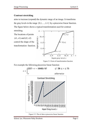
Contrast stretching
aims to increase (expand) the dynamic range of an image. It transforms
the gray levels in the range {0,1,…, L-1} by a piecewise linear function.
The figure below shows a typical transformation used for contrast
stretching.
The locations of points
(r1, s1) and (r2, s2)
control the shape of the
transformation function.
Figure 5.1 Form of transformation function
For example the following piecewise linear function
=
(227 ∗ − 5040)/47 28 ≤ ≤ 75
ℎ
Figure 5.2 Plot of above piecewise linear function
0
15
30
45
60
75
90
105
120
135
150
165
180
195
210
225
240
255
0
15
30
45
60
75
90
105
120
135
150
165
180
195
210
225
240
255
Output
Gray
Level,
s
Input Gray Level, r
Contrast Stretching

will be used to increase the contrast of the image shown in the figure
below:
(a) (b)
(c) (d)
Figure 5.3 Contrast stretching. (a) Original image. (b) Histogram of (a). (c) Result of contrast
stretching. (d) Histogram of (c).
For a given plot, we use the equation of a straight line to compute the
piecewise linear function for each line:
− =
−
−
( − )

For example the plot in Figure 5.2, for the input gray values in the
interval [28 to 75] we get:
− 28 =
255 − 28
75 − 28
( − 28)
= (227 ∗ − 5040)/47 28 ≤ ≤ 75
Similarly, we compute the equations of the other lines.
Another form of contrast stretching is called automatic (full) contrast
stretching as shown in the example below:
=
0 < 90
(255 ∗ − 22950)/48 90 ≤ ≤ 138
255 > 138
Figure 5.4 Full contrast-stretching
This transform produces a high-contrast image from the low-contrast
image as shown in the next figure.
0
51
102
153
204
255
0
15
30
45
60
75
90
105
120
135
150
165
180
195
210
225
240
255
Output
Gray
Level,
s
Input Gray Level, r

(a) (b)
(c) (d)
Figure 5.5 (a) Low-contrast image. (b) Histogram of (a). (c) High-contrast image resulted
from applying full contrast-stretching in Figure 5.4 on (a). (d) Histogram of (c)
Gray-level slicing
Gray-level slicing aims to highlight a specific range [A…B] of gray
levels. It simply maps all gray levels in the chosen range to a high value.
Other gray levels are either mapped to a low value (Figure 5.6(a)) or left
unchanged (Figure 5.6(b)). Gray-level slicing is used for enhancing
features such as masses of water in satellite imagery. Thus it is useful for
feature extraction.

(a) (b)
Figure 5.6 Gray-level slicing
The next figure shows an example of gray level slicing:
(a) Original image
(b) Operation intensifies desired gray level
range, while preserving other values
(c) Result of applying (b) on (a)
(background unchanged)

(d) Operation intensifies desired gray level
range, while changing other values to black
(e) Result of applying (d) on (a) (background
changed to black)
Figure 5.7 Example of gray level slicing
Enhancement through Histogram Manipulation
Histogram manipulation aims to determine a gray-level transform that
produces an enhanced image that has a histogram with desired properties.
We study two histogram manipulation techniques namely Histogram
Equalization (HE) and Histogram Matching (HM).
Histogram Equalization
is an automatic enhancement technique which produces an output
(enhanced) image that has a near uniformly distributed histogram.
For continuous functions, the intensity (gray level) in an image
may be viewed as a random variable with its probability density function
(PDF). The PDF at a gray level r represents the expected proportion
(likelihood) of occurrence of gray level r in the image. A transformation
function has the form

= ( ) = ( − 1) ( )
where w is a variable of integration. The right side of this equation is
called the cumulative distribution function (CDF) of random variable r.
For discrete gray level values, we deal with probabilities (histogram
values) and summations instead of probability density functions and
integrals. Thus, the transform will be:
= ( ) = ( − 1) = ( − 1)
×
=
( − 1)
×
= 0,1,2,… , − 1
The right side of this equation is known as the cumulative histogram for
the input image. This transformation is called histogram equalization or
histogram linearization.
Because a histogram is an approximation to a continuous PDF, perfectly
flat histograms are rare in applications of histogram equalization. Thus,
the histogram equalization results in a near uniform histogram. It spreads
the histogram of the input image so that the gray levels of the equalized
(enhanced) image span a wider range of the gray scale. The net result is
contrast enhancement.

Example:
Suppose that a 3-bit image (L = 8) of size 64 × 64 pixels has the gray
level (intensity) distribution shown in the table below.
r0 = 0
r1 = 1
r2 = 2
r3 = 3
r4 = 4
r5 = 5
r6 = 6
r7 = 7
790
1023
850
656
329
245
122
81
Perform histogram equalization on this image, and draw its normalized
histogram, transformation function, and the histogram of the equalized
image.
Solution:
M × N = 4096
We compute the normalized histogram:
( ) = /
r0 = 0
r1 = 1
r2 = 2
r3 = 3
r4 = 4
r5 = 5
r6 = 6
r7 = 7
790
1023
850
656
329
245
122
81
0.19
0.25
0.21
0.16
0.08
0.06
0.03
0.02

Normalized histogram
Then we find the transformation function:
= ( ) = ( − 1)
= ( ) = 7 = 7 ( ) = 1.33
= ( ) = 7 = 7 ( ) + 7 ( ) = 3.08
and = 4.55, = 5.67, = 6.23, = 6.65, = 6.86, = 7.00
Transformation function
We round the values of s to the nearest integer:
= 1.33 → 1 = 3.08 → 3 = 4.55 → 5
= 5.67 → 6 = 6.23 → 6 = 6.65 → 7
= 6.86 → 7 = 7.00 → 7

These are the values of the equalized histogram. Note that there are only
five gray levels.
( ) = /
r0 = 0
r1 = 1
r2 = 2
r3 = 3
r4 = 4
r5 = 5
r6 = 6
r7 = 7
790
1023
850
656
329
245
122
81
s0 = 1
s1 = 3
s2 = 5
s3 = 6
s4 = 6
s5 = 7
s6 = 7
s7 = 7
790
1023
850
985
448
0.19
0.25
0.21
0.24
0.11
Thus, the histogram of the equalized image can be drawn as follows:
Histogram of equalized image
The next figure shows the results of performing histogram equalization
on dark, light, low-contrast, and high-contrast gray images.

Figure 5.8 Left column original images. Center column corresponding histogram equalized
images. Right column histograms of the images in the center column.

Although all the histograms of the equalized images are different, these
images themselves are visually very similar. This is because the
difference between the original images is simply one of contrast, not of
content.
However, in some cases histogram equalization does not lead to a
successful result as shown below.
(a) Original image (b) Histogram of (a)
Figure 5.9 Image of Mars moon and its histogram
The result of performing histogram equalization on the above image is
shown in the figure below.
(a) Result of applying HE (b) Histogram of (a)
Figure 5.10 Result of applying HE on Figure 5.9 (a)

We clearly see that histogram equalization did not produce a good result
in this case. We see that the intensity levels have been shifted to the upper
one-half of the gray scale, thus giving the image a washed-out
appearance. The cause of the shift is the large concentration of dark
components at or near 0 in the original histogram. In turn, the cumulative
transformation function obtained from this histogram is steep, as shown
in the figure below, thus mapping the large concentration of pixels in the
low end of the gray scale to the high end of the scale.
Figure 5.11 HE transformation function of Figure 5.10(a)
In other cases, HE may introduce noise and other undesired effect to the
output images as shown in the figure below.
(a) Original image (b) Result of applying HE on (a)

(c) Original image (d) Result of applying HE on (c)
Figure 5.12 Undesired effects caused by HE
These undesired effects are a consequence of digitization. When digitize
the continuous operations, rounding leads to approximations.
From the previous examples, we conclude that the effect of HE differs
from one image to another depending on global and local variation in the
brightness and in the dynamic range.
Histogram Matching (Specification)
is another histogram manipulation process which is used to generate a
processed image that has a specified histogram. In other words, it enables
us to specify the shape of the histogram that we wish the processed image
to have. It aims to transform an image so that its histogram nearly
matches that of another given image. It involves the sequential
application of a HE transform of the input image followed by the inverse
of a HE transform of the given image.
The procedure of Histogram Specification is as follows:
1. Compute the histogram ( ) of the input image, and use it to find
the histogram equalization transformation using

= ( ) = ( − 1) = ( − 1)
×
=
( − 1)
×
= 0,1,2, … , − 1
Then round the resulting values, , to the integer range [0, L-1].
2. Compute the specified histogram ( ) of the given image, and use
it find the transformation function G using
( ) = ( − 1) ( ) = 0,1,2, … , − 1
Then round the values of G to integers in the range [0, L-1]. Store
the values of G in a table.
3. Perform inverse mapping. For every value of , use the stored
values of G from step 2 to find the corresponding value of so
that ( ) is closest to and store these mappings from to .
When more than one value of satisfies the given (i.e. the
mapping is not unique), choose the smallest value.
4. Form the output image by first histogram-equalizing the input
image and then mapping every equalized pixel value, , of this
image to the corresponding value in the histogram-specified
image using the inverse mappings in step 3.

Example:
Suppose the 3-bit image of size 64 × 64 pixels with the gray level
distribution shown in the table, and the specified histogram below.
r0 = 0
r1 = 1
r2 = 2
r3 = 3
r4 = 4
r5 = 5
r6 = 6
r7 = 7
790
1023
850
656
329
245
122
81
Perform histogram specification on the image, and draw its normalized
histogram, specified transformation function, and the histogram of the
output image.
Solution:
Step 1:
M × N = 4096
We compute the normalized histogram:
( ) = /
r0 = 0
r1 = 1
r2 = 2
r3 = 3
r4 = 4
r5 = 5
r6 = 6
r7 = 7
790
1023
850
656
329
245
122
81
0.19
0.25
0.21
0.16
0.08
0.06
0.03
0.02

Normalized histogram
Then we find the histogram-equalized values:
= ( ) = ( − 1)
= ( ) = 7 = 7 ( ) = 1.33
= ( ) = 7 = 7 ( ) + 7 ( ) = 3.08
and = 4.55, = 5.67, = 6.23, = 6.65, = 6.86, = 7.00
We round the values of s to the nearest integer:
= 1.33 → 1 = 3.08 → 3 = 4.55 → 5
= 5.67 → 6 = 6.23 → 6 = 6.65 → 7
= 6.86 → 7 = 7.00 → 7
Step 2:
We compute the values of the transformation G

( ) = 7 ( ) = 0
( ) = 7 ( ) = 7[ ( ) + ( )] = 0
and ( ) = 0 , ( ) = 1.05 , ( ) = 2.45
( ) = 4.55 , ( ) = 5.95 , ( ) = 7.00
We round the values of G to the nearest integer:
( )
z0 = 0
z1 = 1
z2 = 2
z3 = 3
z4 = 4
z5 = 5
z6 = 6
z7 = 7
0
0
0
1
2
5
6
7
Transformation function obtained
from the specified histogram
Step 3:
We find the corresponding value of so that the value ( ) is the
closest to .
1
3
5
6
7
3
4
5
6
7

Step 4:
( ) = /
r0 = 0
r1 = 1
r2 = 2
r3 = 3
r4 = 4
r5 = 5
r6 = 6
r7 = 7
790
1023
850
656
329
245
122
81
s0 = 3
s1 = 4
s2 = 5
s3 = 6
s4 = 6
s5 = 7
s6 = 7
s7 = 7
790
1023
850
985
448
0.19
0.25
0.21
0.24
0.11
Thus, the histogram of the output image can be drawn as follows:
To see an example of histogram specification we consider again the
image below.
(a) Original image (b) Histogram of (a)
Figure 5.13 Image of Mars moon and its histogram

We use the following specified histogram shown in the figure below to
perform histogram specification on the image in the previous figure.
Figure 5.14 Specified histogram for image in Figure 5.13(a)
The output image of histogram specification is shown below.
(a) Result of applying HS (b) Histogram of (a)
Figure 5.15 Result of applying HS on Figure 5.13 (a)

DIP_Lecture5.pdf

Recommended

Recommended

More Related Content

Similar to DIP_Lecture5.pdf

Similar to DIP_Lecture5.pdf (20)

Recently uploaded

Recently uploaded (20)

DIP_Lecture5.pdf