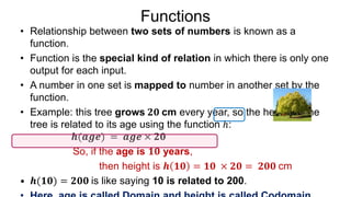
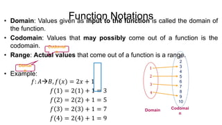
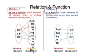
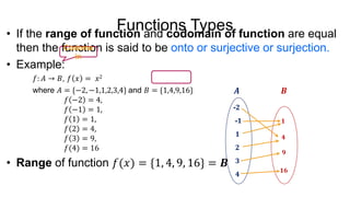
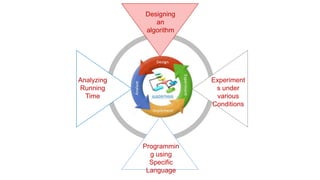
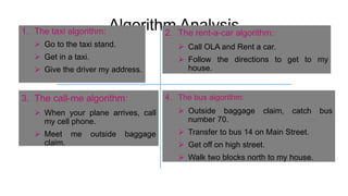
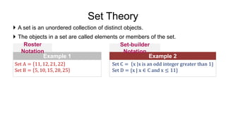
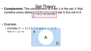
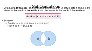
Unit-1 Basic Concept of Algorithm.pptx

Unit-1
Introduction to Algorithm

Designing
an
algorithm
Analyzing
Running
Time
Programmin
g using
Specific
Language
Experiment
s under
various
Conditions

Algorithm Analysis
1. The taxi algorithm:
 Go to the taxi stand.
 Get in a taxi.
 Give the driver my address.
3. The call-me algorithm:
 When your plane arrives, call
my cell phone.
 Meet me outside baggage
claim.
2. The rent-a-car algorithm:
 Call OLA and Rent a car.
 Follow the directions to get to my
house.
4. The bus algorithm:
 Outside baggage claim, catch bus
number 70.
 Transfer to bus 14 on Main Street.
 Get off on high street.
 Walk two blocks north to my house.

 Looping
Outline
 Introduction to Algorithm
• Definition
• Characteristics
• Types
• Simple Multiplication Methods
 Mathematics for Algorithmic Sets
• Set Theory
• Functions and Relations
• Vectors and Matrices
• Linear Inequalities and Linear Equations
• Logic and Quantifiers

What is an Algorithm?
Output
Input Process
Ingredient
s
Recip
e
Cak
e

What is an Algorithm?
Output
Algorithm Program
Input

Characteristics of An Algorithm

Simple Multiplication Methods
1. American
approach
2. English approach
9 8 1
3 9 2 4
2 9 4 3
1 9 6 2
9 8 1
1 2 1 0 5 5
4
4
3
2
1
9 8 1
3 9 2 4
2 9 4 3
1 9 6 2
9 8 1
1 2 1 0 5 5
4
4
3
2
1

3. à 𝒍𝒂 𝒓𝒖𝒔𝒔𝒆 multiplication
i. Write the multiplicand and multiplier side by side.
ii. Make two columns, one under each operand.
iii. Repeat step iv and v until the number in the left
column is 1.
iv. Divide the number in the left hand column by 2,
ignoring any fractions.
v. Double the number in the right hand column by adding
it to itself.
vi. Next cross out each row where the number in the left
hand column is even.
vii. Finally add up the numbers that remain in the right
hand column.
1234
2468
4936
9872
19744
39488
78976
157952
315904
631808
981
490
245
122
61
30
15
7
3
1
1234
4936
19744
78976
157952
315904
631808
1210554

4. Multiplication by divide and conquer
• Both the multiplicand and the multiplier must have the same number of digits
and this number be a power of 2. If not then it can be done by adding zeros
on the left if necessary.
Multiply Shift Result
(09) * (12) 4
(09) * (34) 2
(81) * (12) 2
(81) * (34) 0
. .
.
.
8
0
1
. .
6
0
3
. .
2
7
9
5 4
7
2
1 2 1 0 5 5 4
Multiplier 1 2 3 4
Multiplicand 0 9 8 1
i. Multiply left half of the multiplicand by left half of multiplier
and shift the result by no. of digits of multiplier i.e. 4.
ii. Multiply left half of the multiplicand by right half of the
multiplier, shift the result by half the number of digits of
multiplier i.e. 2.
iii. Multiply right half of the multiplicand by left half of the
multiplier, shift the result by half the number of digits of
multiplier i.e. 2.
iv. Multiply right half of the multiplicand by right half of the
multiplier the result is not shifted at all.

Set Theory
 A set is an unordered collection of distinct objects.
 The objects in a set are called elements or members of the set.
Example 1
Set A = 11, 12, 21, 22
Set B = 5, 10, 15, 20, 25
Set C = x x is an odd integer greater than 1}
Set D = {x | x ∈ C and x ≤ 11}
Example 2
Roster
Notation
Set-builder
Notation

Set Theory
Example 1
A = 𝑥 𝑥 ∈ Z and 𝑥2 − 81 = 0}
A = −9,9
B = 𝑥 𝑥 is divisible by 2}
B = {2,4,6, … , }
Example 2
Set 𝐀 is a finite
set
Set 𝐁 is an infinite
set

Set Theory
Example 1
If 𝐴 = {1,3,5} and 𝐵 = 1,5
Then set 𝐵 is a proper subset of
𝐴.
If 𝐴 = {1,3,5} and 𝐶 = 1,3,5
Then set C is a subset of 𝐴, but it is
not a proper subset of 𝐴 since 𝐶 =
𝐴.
Example 2
A=
C
𝑩⊂𝑨 𝑪 ⊆ 𝑨
A

Set Theory
• Complement: The complement of a set 𝐴 is the set 𝐴’ that
contains every element of the Universal set U but not in A.
• Example:
– Consider 𝑈 = {1, 3, 5, 7, 9} and 𝐴 = 1, 5
Then 𝐴′ = {3, 7, 9}
U
A
A
’
𝐴′ = {𝑥 | 𝑥 ∈𝑈 𝑎𝑛𝑑 𝑥∉𝐴
}

Set Operations
A B
A B
𝑨 ∪ 𝑩 = {𝒙 | 𝒙 ∈ 𝑨 𝒐𝒓 𝒙 ∈ 𝑩}

Set Operations
 Intersection: The intersection of two sets 𝐴 and 𝐵 is the set that contains all
elements of 𝐴 that also belong to 𝐵 but no other elements.
 Example:
 Consider 𝐴 = {1, 3, 5, 7, 9} and 𝐵 = {1, 2, 3, 4, 5}
Then 𝐴 ∩ 𝐵 = {1, 3, 5}
A B
𝑨 ∩ 𝑩 = {𝒙 | 𝒙 ∈ 𝑨 𝒂𝒏𝒅 𝒙 ∈ 𝑩}

Set Operations
• Set Difference: The set difference 𝐴 − 𝐵 of two sets 𝐴 and 𝐵
is the set of elements that are in 𝑨 but not in 𝑩.
• Example:
– Consider 𝐴 = {1, 3, 5, 7, 9} and 𝐵 = {1, 2, 3, 4, 5}
Then 𝐴 − 𝐵 = {7, 9}
A B
𝑨 – 𝑩 = {𝒙 | 𝒙 ∈ 𝑨 𝒂𝒏𝒅 𝒙 ∉ 𝑩}

Set Operations
 Symmetric Difference: The symmetric difference 𝐴 ⊖ 𝐵 of two sets 𝐴 and 𝐵 is the
elements that are in 𝑨 but not in 𝑩 and the elements that are in 𝑩 but not in 𝑨.
 Example:
 Consider, 𝐴 = {1, 3, 5, 7, 9} and 𝐵 = {1, 2, 3, 4, 5}
Then 𝐴 ⊖ 𝐵 = {7, 9, 2, 4}
A B
𝑨 – 𝑩 = {𝒙 | 𝒙 ∈ 𝑨 𝒂𝒏𝒅 𝒙 ∉ 𝑩}

Set Operations
𝐴
{1,2,3}
𝐵
{𝑥, 𝑦}
(1, 𝑥) (1, 𝑦)
(2, 𝑥) (2, 𝑦)
(3, 𝑥) (3, 𝑦)
𝐴 × 𝐵
𝑨 × 𝑩 = {(𝒂, 𝒃) | 𝒂 ∈ 𝑨 𝒂𝒏𝒅 𝒃 ∈ 𝑩}

Properties of the Relation
• Reflexive: Let 𝐴 be a set, and let 𝑅 be a binary relation on 𝐴.
Relation 𝑅 is reflexive if,
Example 1
A = {1, 2} and R1 = {(a, b) | a ≤ b}
so, R1 = 1,1 , 1,2 , 2,2
B = 1,2,3 , and
R2 = {(1,1), (1,2), (2,1), (2,2), (3,1)}
Example 2
Reflexive
Not Reflexive since (𝟑, 𝟑) ∉
𝑹
∀𝒙: [(𝒙 ∈ 𝑨) → ((𝒙, 𝒙) ∈ 𝑹)]

• Symmetric: A relation 𝑅 on a set 𝐴 is called symmetric if
(𝑦, 𝑥) ∈ 𝑅 whenever (𝑥, 𝑦) ∈ 𝑅, for some 𝑥, 𝑦 ∈ 𝐴.
Example 1
A = {1,2,3} and R1 = {(a, b)|a ≠ b}
R1 = {(1,2), (1,3), (2,1), (2,3), (3,1), (3,2)}
B = { 1, 2, 3} and R2 = {(a, b) | a ≤ b}
So, R2 = {(1,1), (1,2), (1,3), (2,2), (2,3), (3,3)}
Example 2
Symmetri
c
Asymmetri
c
∀𝒙: ∀𝒚: [((𝒙, 𝒚) ∈ 𝑹) → ((𝒚, 𝒙) ∈ 𝑹)]

• Transitive: A relation 𝑅 on a set 𝐴, is called transitive if
whenever (𝑥, 𝑦) ∈ 𝑅 and (𝑦, 𝑧) ∈ 𝑅, then (𝑥, 𝑧) ∈ 𝑅, for 𝑥, 𝑦, 𝑧 ∈
𝐴.
Example 1
A = { 1, 2, 3} and R1 = {(a, b) | a ≤ b}
So, R1 =
{(1,1), (1,2), (1,3), (2,2), (2,3), (3,3)}
B = 1, 2, 3,4 and
R2 = a, b | 𝑤ℎ𝑒𝑟𝑒 𝑏 𝑖𝑠 𝑎 𝑠𝑢𝑐𝑐𝑒𝑠𝑠𝑜𝑟 𝑜𝑓 𝑎
So, R2 = { 1,2 , 2,3 , (3,4)}
Example 2
Transitive
∀𝒙: ∀𝒚: ∀𝒛[([(𝒙, 𝒚) ∈ 𝑹] ∧ [(𝒚, 𝒛) ∈ 𝑹]) → ((𝒙, 𝒛) ∈ 𝑹)]
Not
Transitive

Functions
• Relationship between two sets of numbers is known as a
function.
• Function is the special kind of relation in which there is only one
output for each input.
• A number in one set is mapped to number in another set by the
function.
• Example: this tree grows 𝟐𝟎 cm every year, so the height of the
tree is related to its age using the function ℎ:
𝒉(𝒂𝒈𝒆) = 𝒂𝒈𝒆 × 𝟐𝟎
So, if the age is 𝟏𝟎 years,
then height is 𝒉 𝟏𝟎 = 𝟏𝟎 × 𝟐𝟎 = 𝟐𝟎𝟎 cm
• 𝒉(𝟏𝟎) = 𝟐𝟎𝟎 is like saying 10 is related to 200.

Function Notations
• Domain: Values given as input to the function is called the domain of
the function.
• Codomain: Values that may possibly come out of a function is the
codomain.
• Range: Actual values that come out of a function is a range.
• Example:
𝑓: 𝐴𝐵, 𝑓(𝑥) = 2𝑥 + 1
𝑓(1) = 2(1) + 1 = 3
𝑓(2) = 2(2) + 1 = 5
𝑓 3 = 2 3 + 1 = 7
𝑓(4) = 2(4) + 1 = 9
Domain Codomai
n
1
2
3
4
1
2
3
4
5
6
7
8
9
10
Codomai
n
Domai
n

Relation & Function
Division
(Domain)
Students
(Codomain)
CX
CY
CZ
Ana
Mit
Sa
m
Yug
Jen
To
m
Ra
m
Nee
l
Is not a function since elements
of domain point to multiple
elements of codomain.
Relation 1
Is a function since elements of
domain point to only one element
of codomain.
Relation 2
Ana
Yug
Ra
m
Mit
CX
CY
CZ
Division
(Codomain)
Students
(Domain)

Functions Types
• If the range of function and codomain of function are equal
then the function is said to be onto or surjective or surjection.
• Example:
𝑓: 𝐴 → 𝐵, 𝑓 𝑥 = 𝑥2
where 𝐴 = {−2, −1,1,2,3,4} and 𝐵 = {1,4,9,16}
𝑓 −2 = 4,
𝑓 −1 = 1,
𝑓 1 = 1,
𝑓 2 = 4,
𝑓 3 = 9,
𝑓(4) = 16
• Range of function 𝑓(𝑥) = {1, 4, 9, 16} = 𝑩
𝑨 𝑩
𝟏
𝟐
𝟑
𝟒
𝟏
𝟒
𝟗
𝟏𝟔
-𝟐
-𝟏
Codoma
in

Functions Types
𝟐
𝟑
𝟒
𝟓
𝟏
𝟐
𝟑
𝟒
𝑨 𝑩

Functions Types
𝐁
1
2
3
4
1
4
9
16
𝑨

Linear Equations
𝒂𝒙 = 𝒃 𝒙 =
𝒃
𝒂
Solution

Logical Connectives
• Conjunction (Ʌ):
The logical
connective
Conjunction (logical
AND) is true only
when both of the
propositions are
true.
• Example:
𝑝 : It is raining
𝑞 : It is cold
𝑟 : It is raining AND it is
𝒑 𝒒 𝒓 =
𝒑 Ʌ 𝒒
𝑇𝑟𝑢𝑒 𝑇𝑟𝑢𝑒
𝑇𝑟𝑢𝑒 𝐹𝑎𝑙𝑠𝑒
𝐹𝑎𝑙𝑠𝑒 𝑇𝑟𝑢𝑒
𝐹𝑎𝑙𝑠𝑒 𝐹𝑎𝑙𝑠𝑒
𝑇𝑟𝑢𝑒
𝐹𝑎𝑙𝑠𝑒
 Disjunction (V): The
logical disjunction, or
logical OR, is true if one
or both of the
propositions are true.
 Example:
p ∶ 2 + 2 = 5
q ∶ 1 < 2
r ∶ 2 + 2 = 5 𝐎𝐑 1 < 2
 Truth table
𝑝 𝑞 𝑟 = 𝑝 V 𝑞
𝑇𝑟𝑢𝑒 𝑇𝑟𝑢𝑒
𝐹𝑎𝑙𝑠𝑒 𝐹𝑎𝑙𝑠𝑒
𝑇𝑟𝑢𝑒
𝑇𝑟𝑢𝑒
𝑇𝑟𝑢𝑒
 Negation (): 𝑝, the
negation of a
proposition 𝑝, is also a
proposition.
 Example:
p : John studies.
 p : John does
NOT study.
 Truth table
𝑝  𝑝

Logical Quantifiers
• Existential Quantifier (denoted as “” for some): 𝑃(𝑎) is the
preposition, if there exits an element 𝑎 in the universe of
discourse such that 𝑃(𝑎) is giving expected result then the
Existential Quantification of 𝑃(𝑎) is represented by, ∃𝒂 𝑷(𝒂).
• Example:
– Let 𝑃(𝑥) = 𝑥/2 < 𝑥
There exists a numerical value for which 𝑥/2 < 𝑥 is true
Thus,  𝑥 ∶ 𝑃(𝑥) is true
• In order to show an existential quantification is true, it must be
shown true for only ONE value.
• In order to show an existential quantification is false, it must be
show false for ALL values.

Unit-1 Basic Concept of Algorithm.pptx

More Related Content

Similar to Unit-1 Basic Concept of Algorithm.pptx

Recently uploaded

Unit-1 Basic Concept of Algorithm.pptx