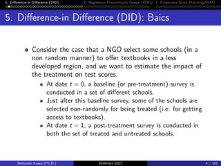
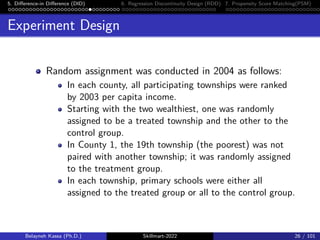
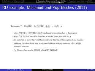
The document discusses the difference-in-differences (DID) method for estimating treatment effects using observational data. It provides an example of a study that used DID to estimate the impact of a minimum wage increase in New Jersey. DID calculates the effect of a treatment by comparing the change over time in outcomes for the treatment group to the control group. A key assumption is that the treatment and control groups would have followed parallel trends in the absence of treatment. The document also discusses how to implement DID using regression analysis and examines its use in a randomized controlled trial that evaluated providing eyeglasses to Chinese students.


![5. Difference-in Difference (DID) 6. Regression Discontinuity Design (RDD) 7. Propensity Score Matching(PSM)
DID; Estimator
The DID estimator is given by:
DD = [E(YT
i1|T) − E(YC
i1|C)] − [E(YC
i0|T) − E(YC
i0|C)]
= [E(YT
i1|T) − E(YC
i0|T)] − [E(YC
i1|C) − E(YC
i0|C)]
= (T1 − T0) − (C1 − C0)
= (CTVCT + TE) − CTVCC,
where CTVCT and CTVCC stand for ”changes in
time-varying characteristics” in the treatment and in the
control group respectively, and TE stands for the
”treatment effect”.
Belayneh Kassa (Ph.D.) Skillmart-2022 7 / 101](https://image.slidesharecdn.com/did-230104062629-1751e43d/85/DID-pdf-7-320.jpg)


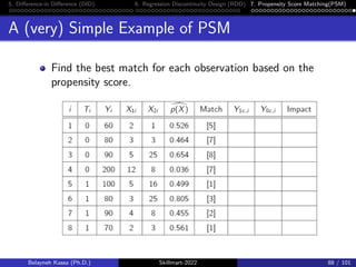
![5. Difference-in Difference (DID) 6. Regression Discontinuity Design (RDD) 7. Propensity Score Matching(PSM)
A (very) Simple Example of PSM
Find counterfactual (comparison) outcomes Yicfor each
non-treated and Y[0c]for each treated.
Belayneh Kassa (Ph.D.) Skillmart-2022 89 / 101](https://image.slidesharecdn.com/did-230104062629-1751e43d/85/DID-pdf-89-320.jpg)