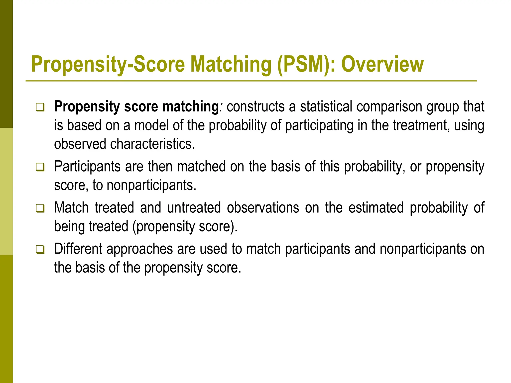
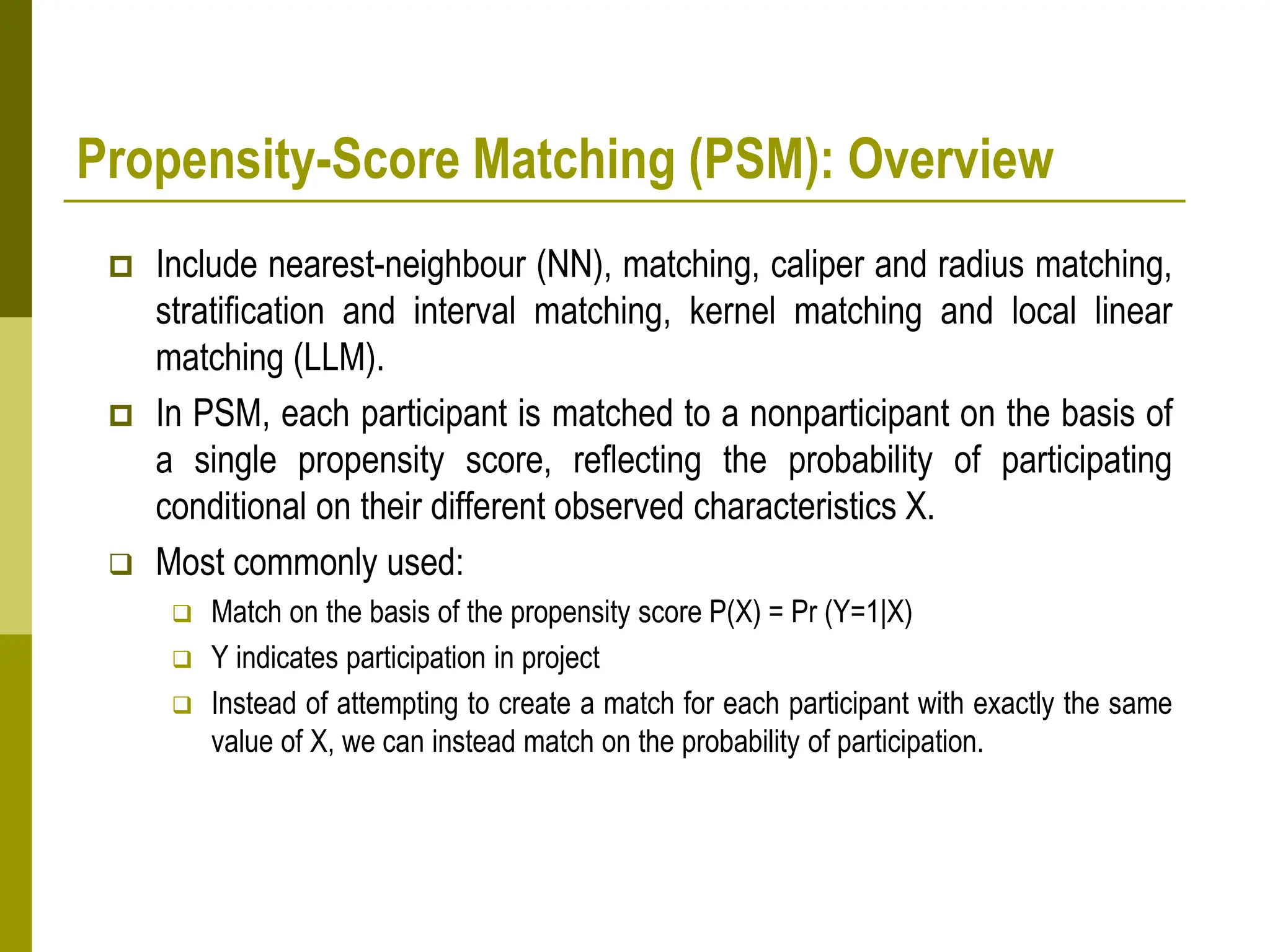
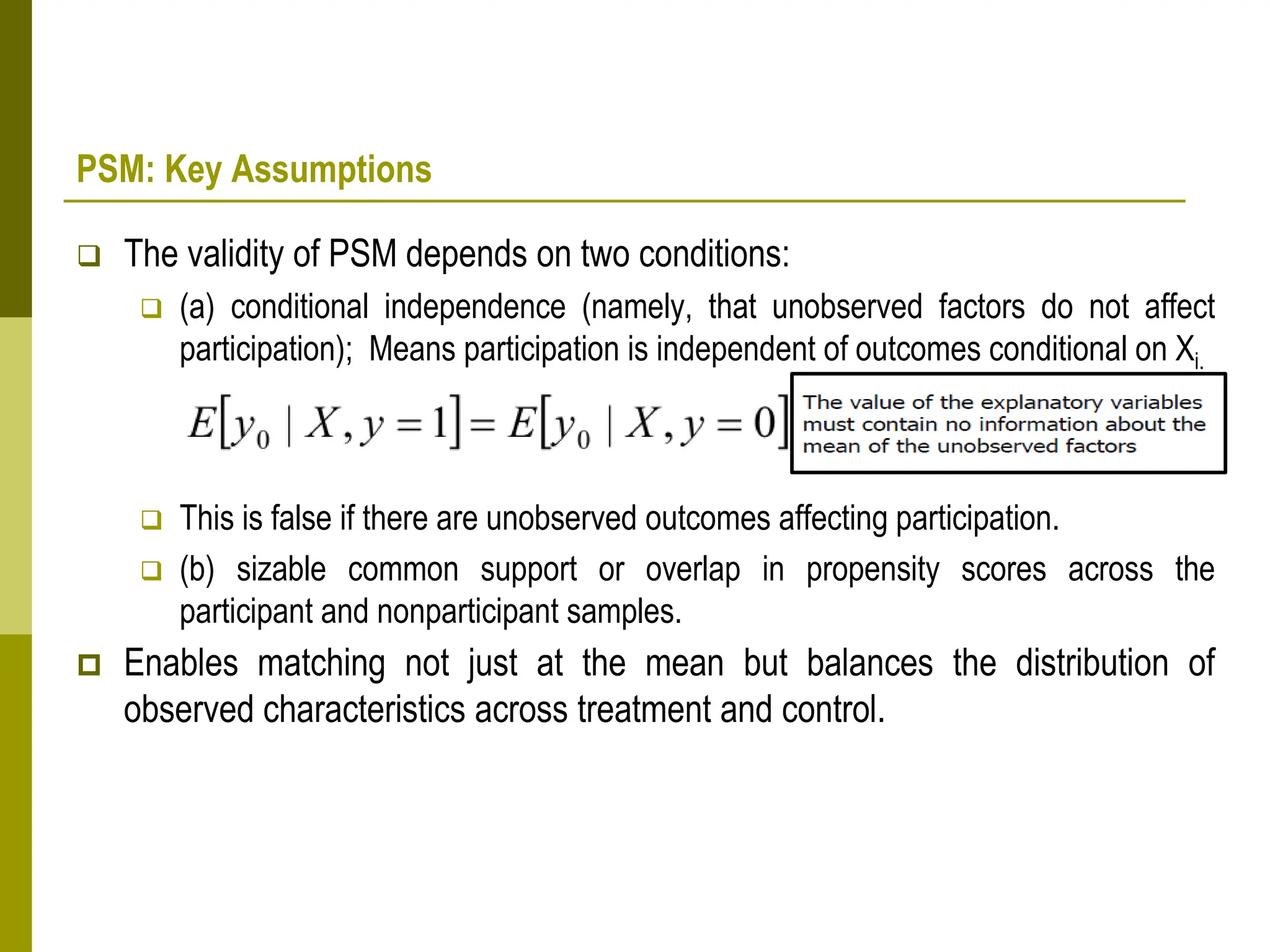
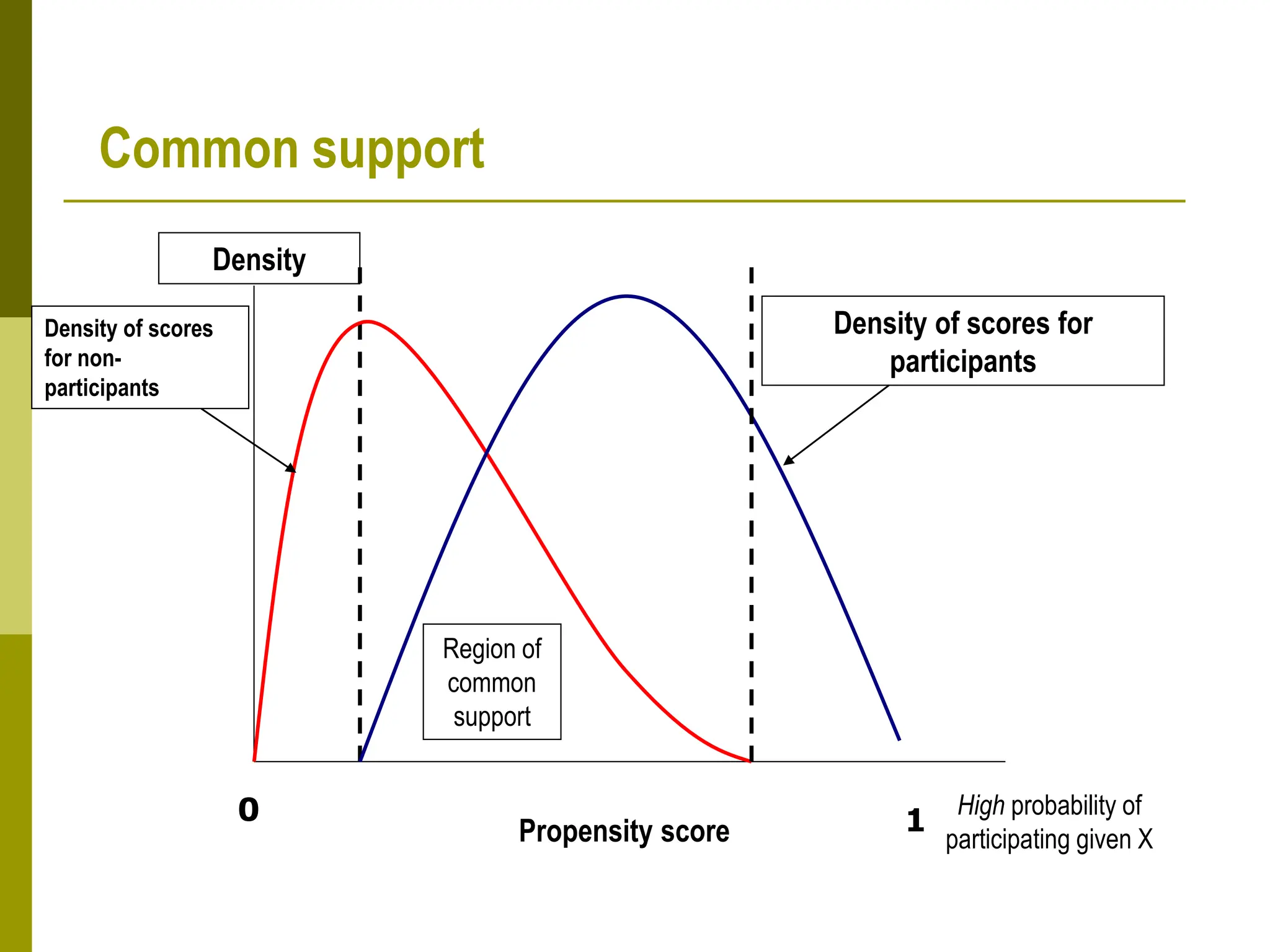
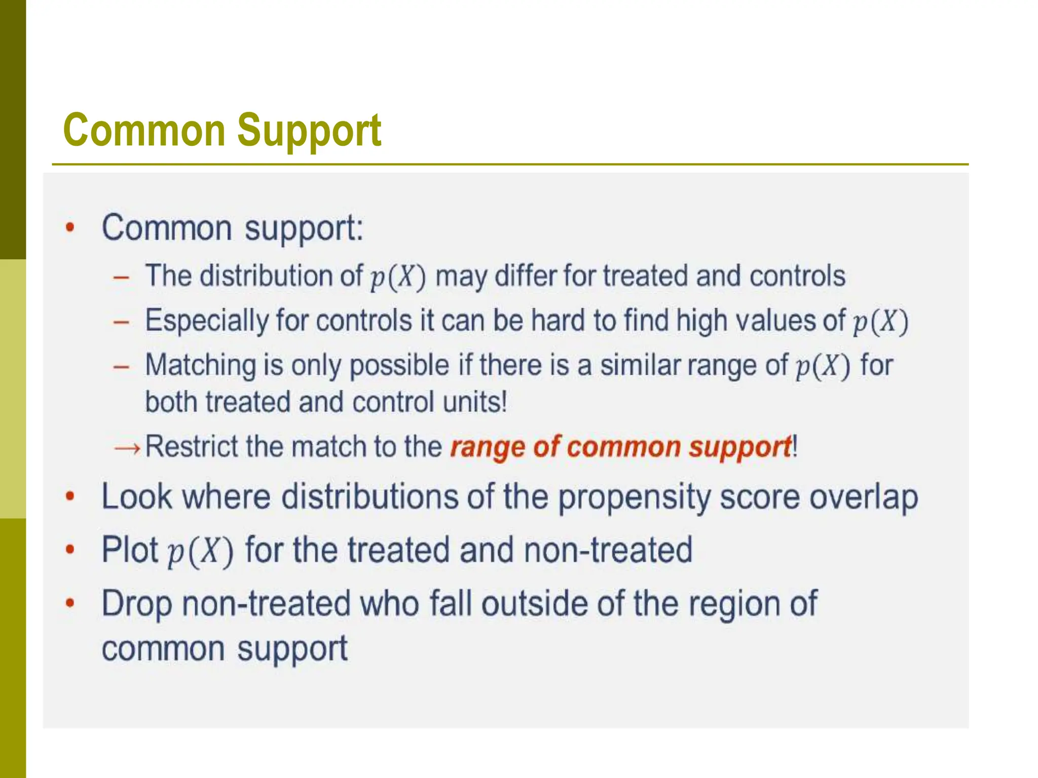
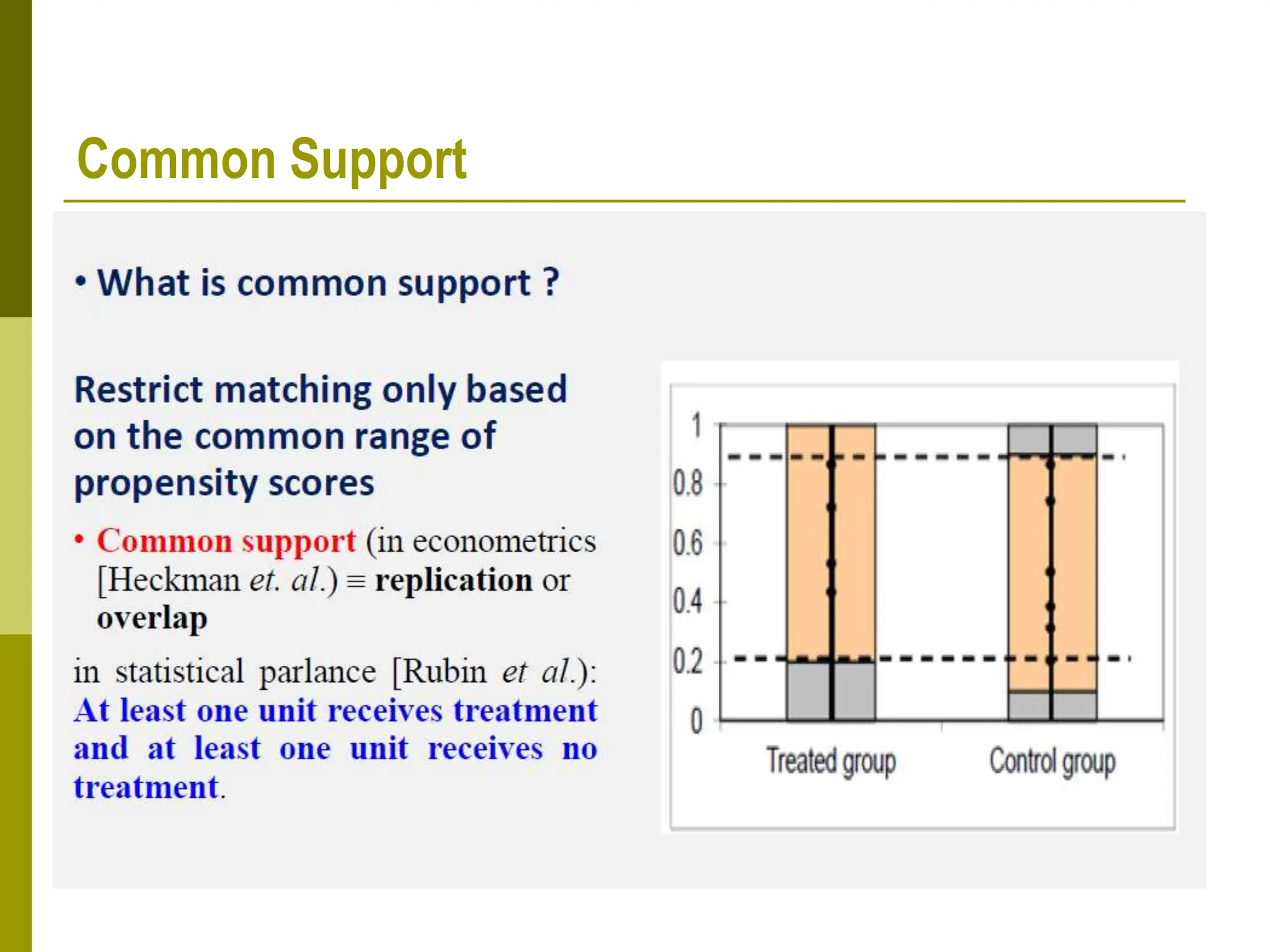
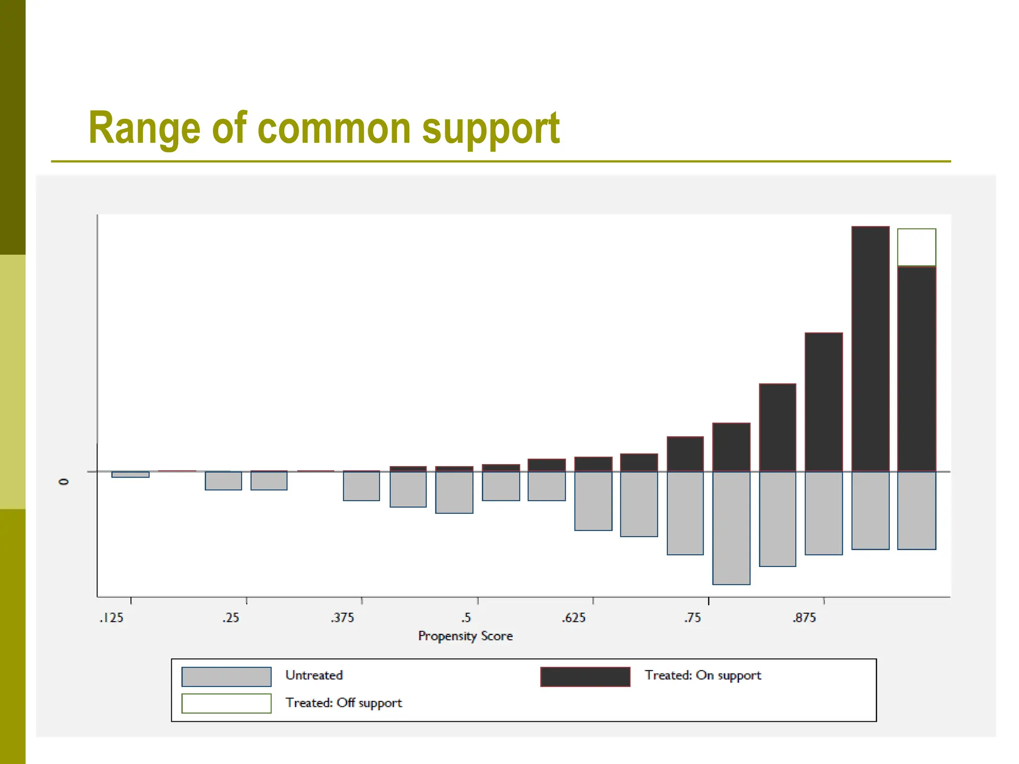
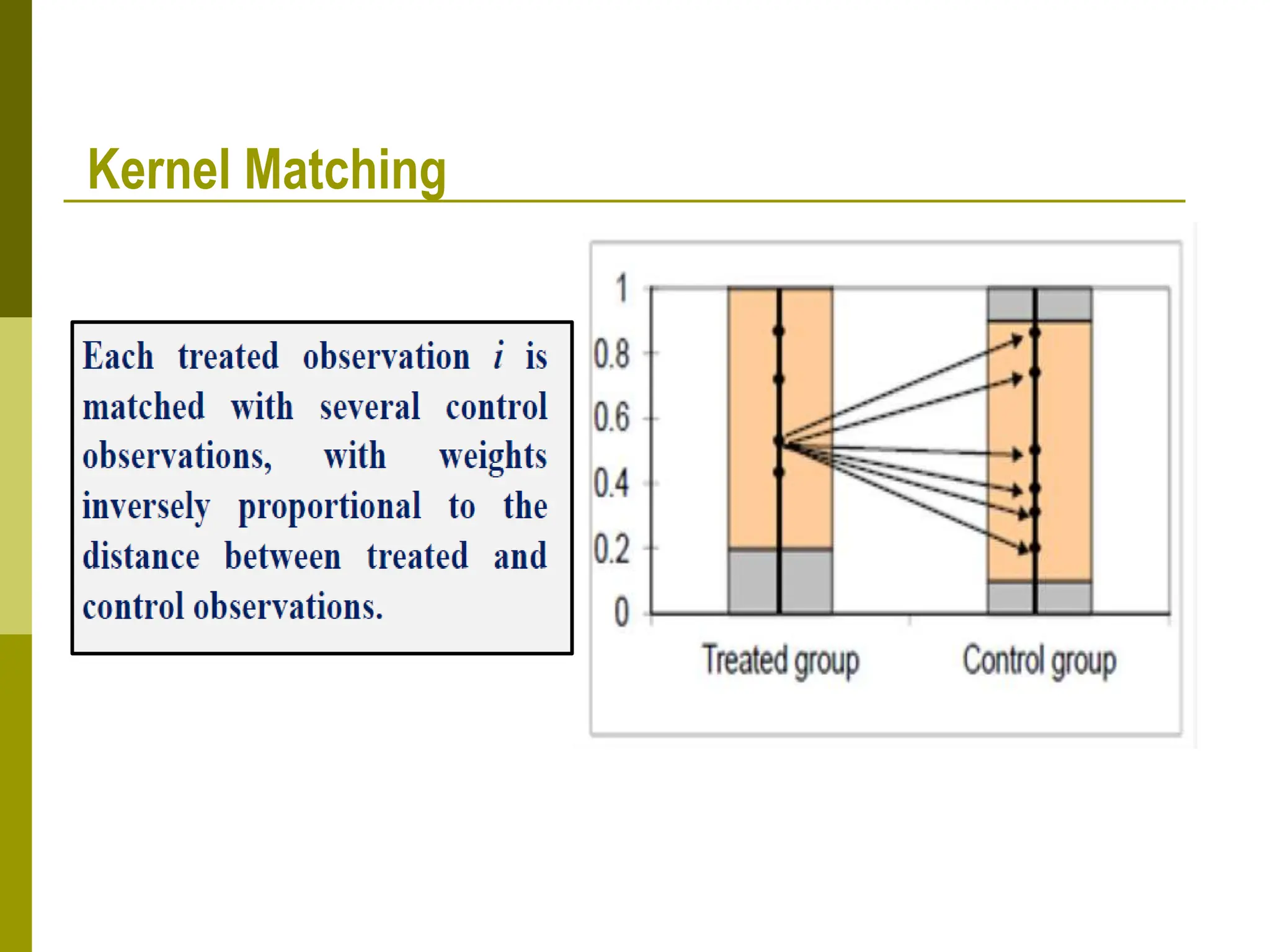
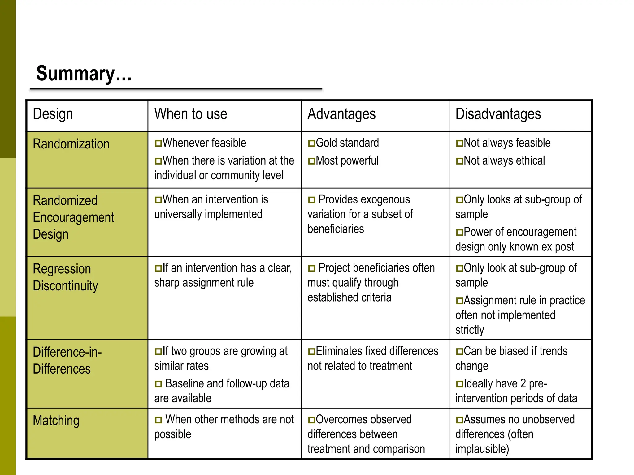
Propensity score matching (PSM) is a statistical technique used to estimate causal treatment effects. It constructs a comparison group that is matched to the treated group based on propensity scores, which represent the probability of participating in a treatment given observed characteristics. Key assumptions of PSM include conditional independence and common support. Different matching methods can then be used such as nearest neighbor matching, caliper matching, and kernel matching. PSM provides a way to control for selection bias and estimate treatment effects when a randomized experiment is not possible. However, it relies on the untestable assumption that selection depends only on observed characteristics.

1. Propensity-Score Matching
(PSM)
Misgina Asmelash, Ph.D.
in Agricultural Economics and Management
YOM Institute of Economic Development
Nov 02, 2018

2. Propensity-Score Matching
(PSM)
The problem with matching is to credibly identify groups that look alike. Identification is a problem
because even if households are matched along a vector, X, of different characteristics, one would
rarely find two households that are exactly similar to each other in terms of many characteristics.
Because many possible characteristics exist, a common way of matching households is
propensity score matching.

3. Propensity-Score Matching (PSM): Overview
 Propensity score matching: constructs a statistical comparison group that
is based on a model of the probability of participating in the treatment, using
observed characteristics.
 Participants are then matched on the basis of this probability, or propensity
score, to nonparticipants.
 Match treated and untreated observations on the estimated probability of
being treated (propensity score).
 Different approaches are used to match participants and nonparticipants on
the basis of the propensity score.

4. Propensity-Score Matching (PSM): Overview
 Include nearest-neighbour (NN), matching, caliper and radius matching,
stratification and interval matching, kernel matching and local linear
matching (LLM).
 In PSM, each participant is matched to a nonparticipant on the basis of
a single propensity score, reflecting the probability of participating
conditional on their different observed characteristics X.
 Most commonly used:
 Match on the basis of the propensity score P(X) = Pr (Y=1|X)
 Y indicates participation in project
 Instead of attempting to create a match for each participant with exactly the same
value of X, we can instead match on the probability of participation.

5. PSM: Key Assumptions
 The validity of PSM depends on two conditions:
 (a) conditional independence (namely, that unobserved factors do not affect
participation); Means participation is independent of outcomes conditional on Xi.
 This is false if there are unobserved outcomes affecting participation.
 (b) sizable common support or overlap in propensity scores across the
participant and nonparticipant samples.
 Enables matching not just at the mean but balances the distribution of
observed characteristics across treatment and control.

6. Density
0 1
Propensity score
Region of
common
support
Density of scores for
participants
High probability of
participating given X
Density of scores
for non-
participants
Common support

7. Common Support

8. Common Support

9. Range of common support

10. Nearest Neighbor Matching

11. Which Neighbor?

12. Which Neighbor?

13. Caliper Matching

14. Kernel Matching

15. Kernel Matching

16. Steps in Score Matching
1. Need representative and comparable data for both treatment and
comparison groups.
2. Use a logit (or other discrete choice model) to estimate program
participations as a function of observable characteristics.
3. Use predicted values from logit to generate propensity score p(xi) for all
treatment and comparison group members
4. Match Pairs:
 Restrict sample to common support (as in Figure).
 Need to determine a tolerance limit: using matching methods, Such as:
 Nearest neighbors (NN), caliper and radius matching, kernel matching and
weighting by the propensity score.
5. Once matches are made, we can calculate impact by comparing the
means of outcomes across participants and their matched pairs.

17. PSM vs. Randomization
 Randomization does not require the untestable assumption of
independence conditional on observables.
 PSM requires large samples and good data:
1. Ideally, the same data source is used for participants and non-
participants
2. Participants and non-participants have access to similar institutions
and markets, and
3. The data include X variables capable of identifying program
participation and outcomes.

18. Lessons on Matching Methods
 Typically used when neither randomization or other quasi experimental
options are not possible.
 Case 1: no baseline. Can do ex-post matching
 Dangers of ex-post matching:
 Matching on variables that change due to participation (i.e., endogenous)
 Matching helps control only for OBSERVABLE differences, not
unobservable differences.
 Matching becomes much better in combination with other techniques, such
as:
 Exploiting baseline data for matching and using difference-in-difference
strategy
 If an assignment rule exists for project, can match on this rule
 Need good quality data: common support can be a problem if two groups
are very different.

19. Design When to use Advantages Disadvantages
Randomization Whenever feasible
When there is variation at the
individual or community level
Gold standard
Most powerful
Not always feasible
Not always ethical
Randomized
Encouragement
Design
When an intervention is
universally implemented
 Provides exogenous
variation for a subset of
beneficiaries
Only looks at sub-group of
sample
Power of encouragement
design only known ex post
Regression
Discontinuity
If an intervention has a clear,
sharp assignment rule
 Project beneficiaries often
must qualify through
established criteria
Only look at sub-group of
sample
Assignment rule in practice
often not implemented
strictly
Difference-in-
Differences
If two groups are growing at
similar rates
 Baseline and follow-up data
are available
Eliminates fixed differences
not related to treatment
Can be biased if trends
change
Ideally have 2 pre-
intervention periods of data
Matching  When other methods are not
possible
Overcomes observed
differences between
treatment and comparison
Assumes no unobserved
differences (often
implausible)
Summary…