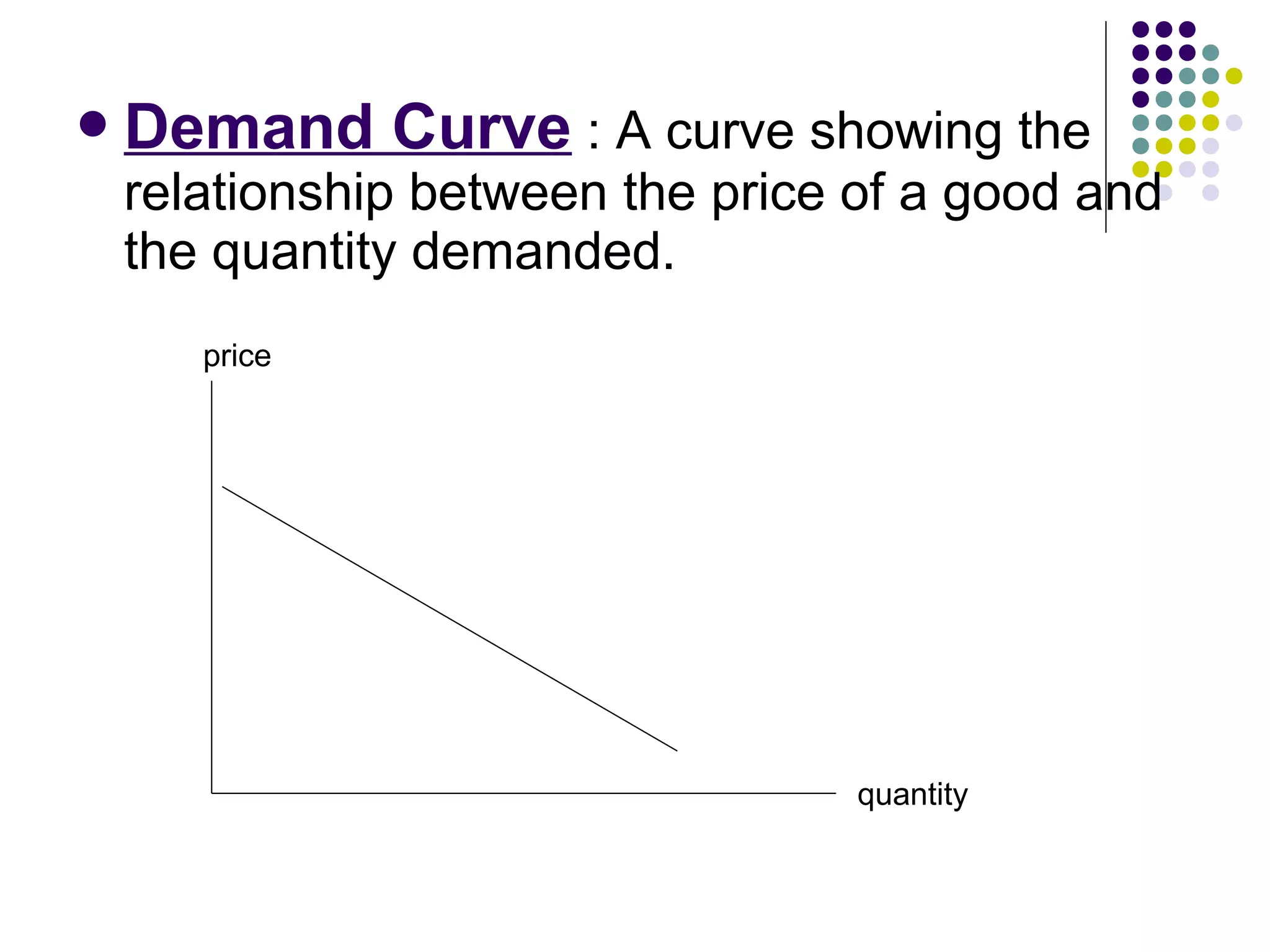
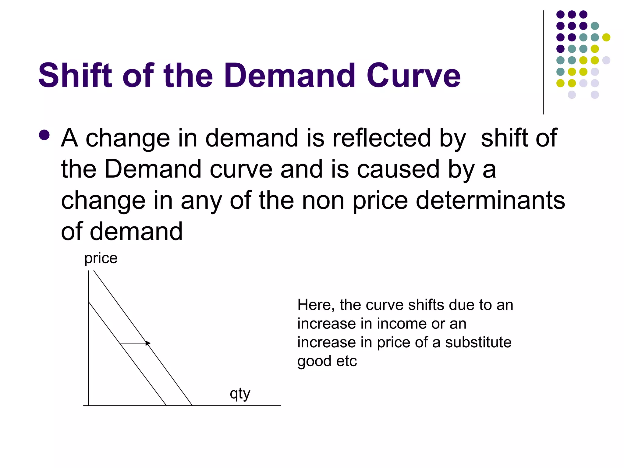
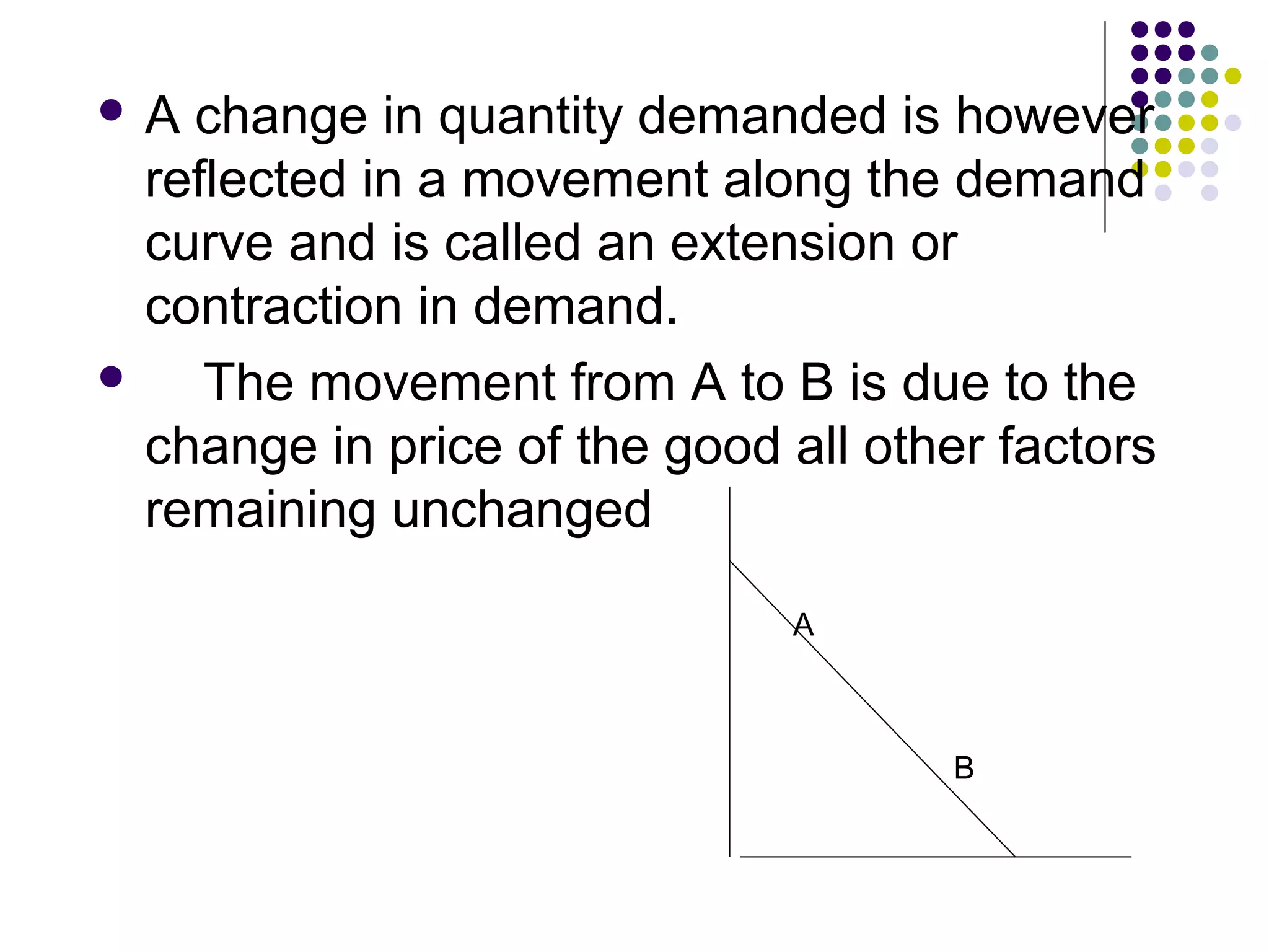
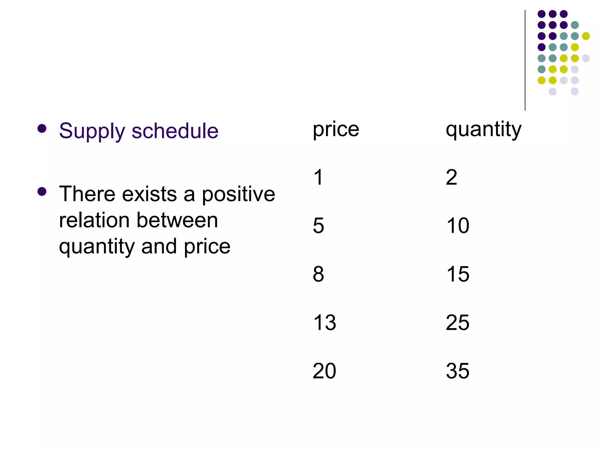
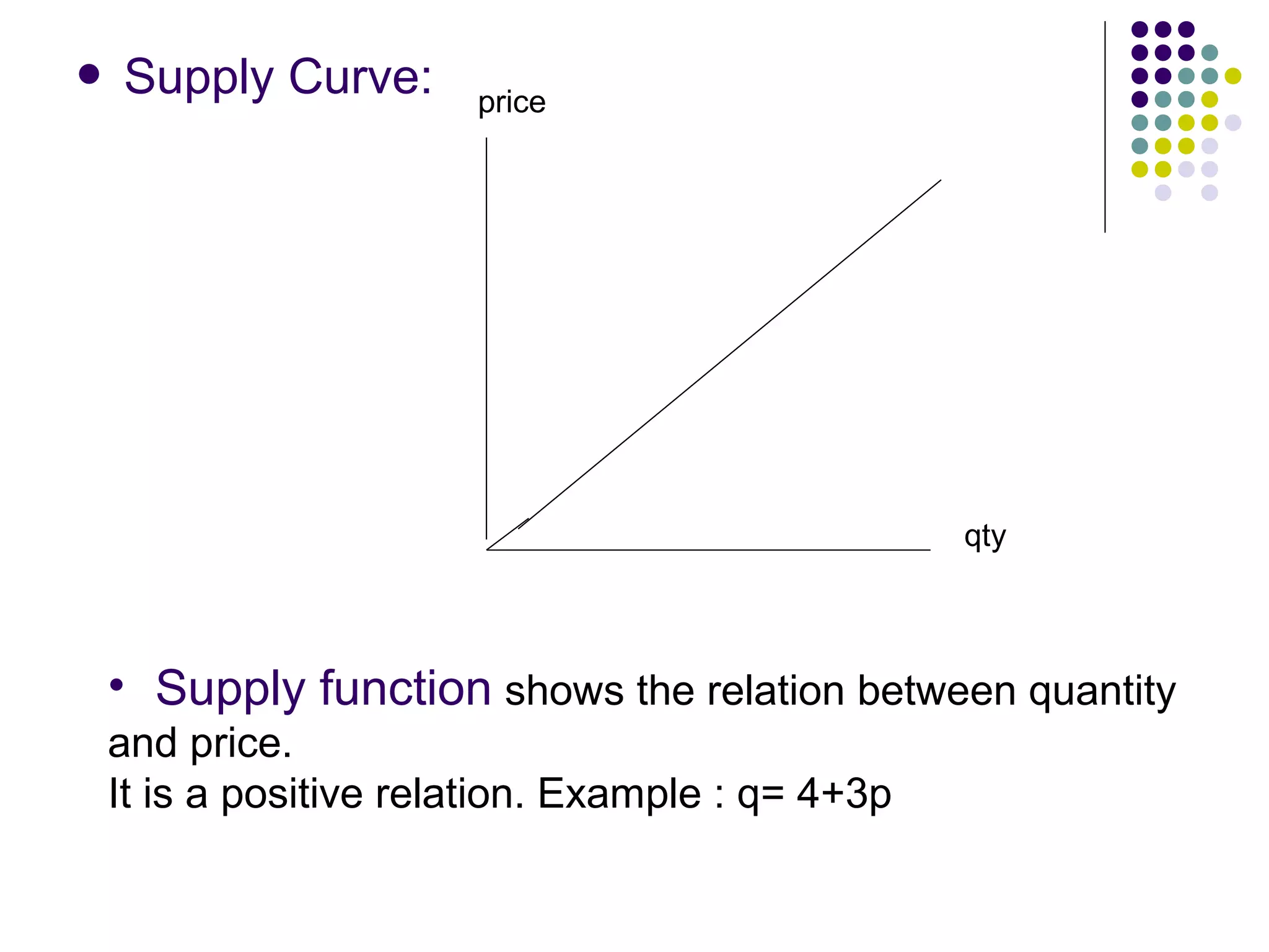
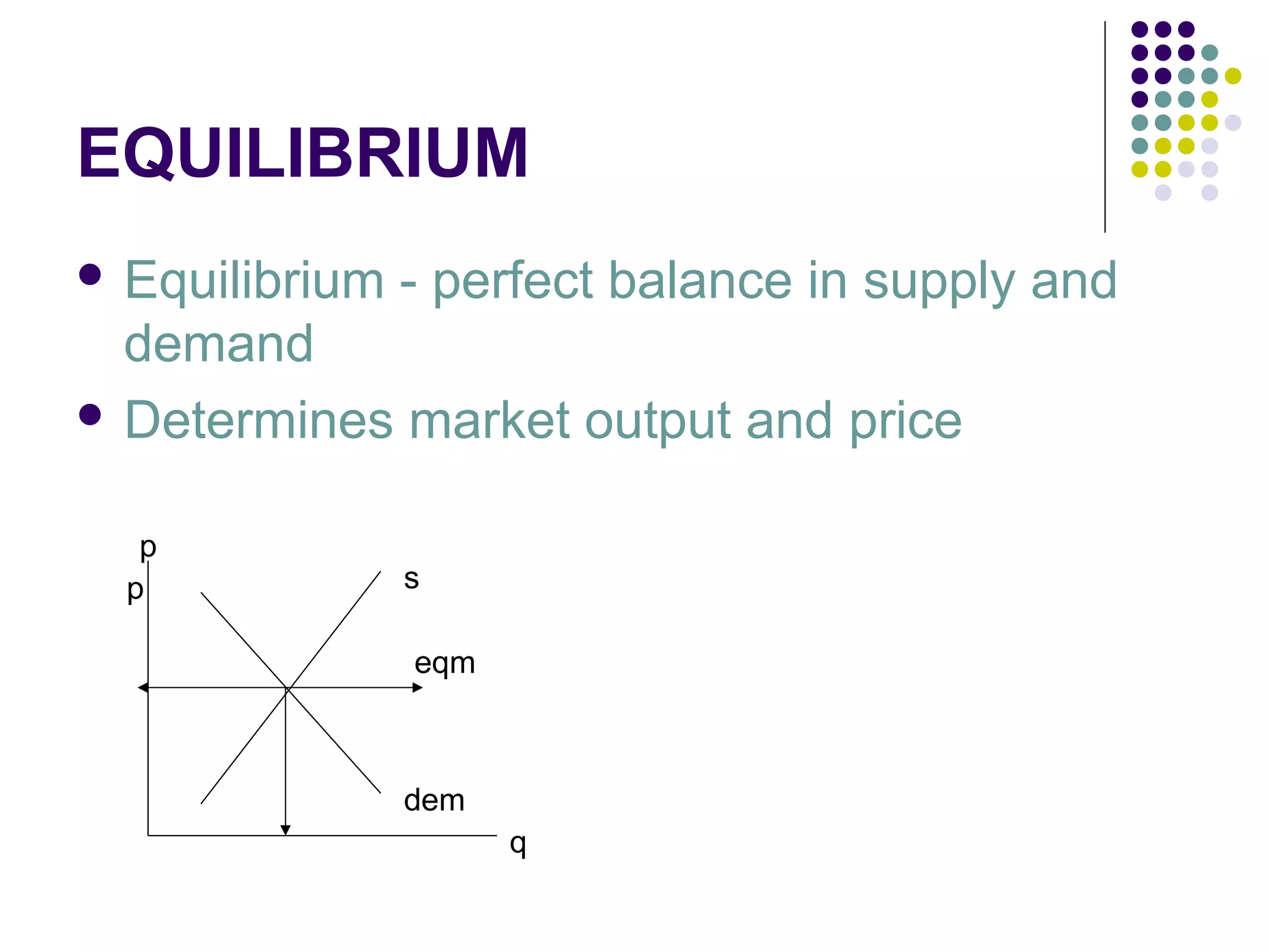
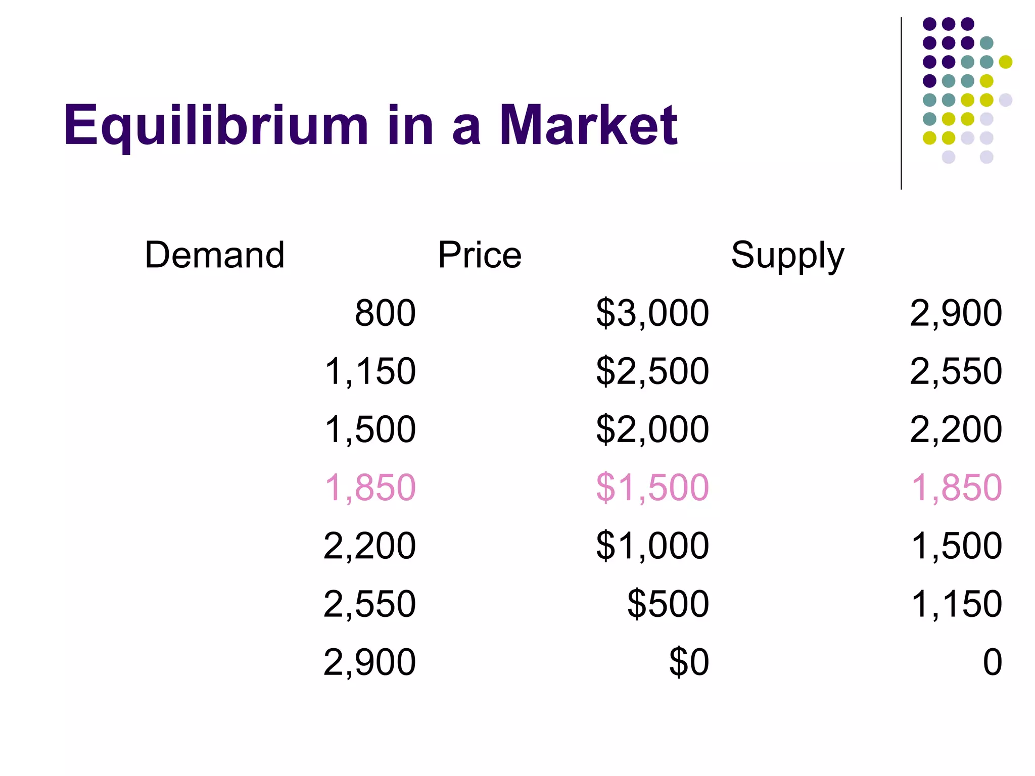
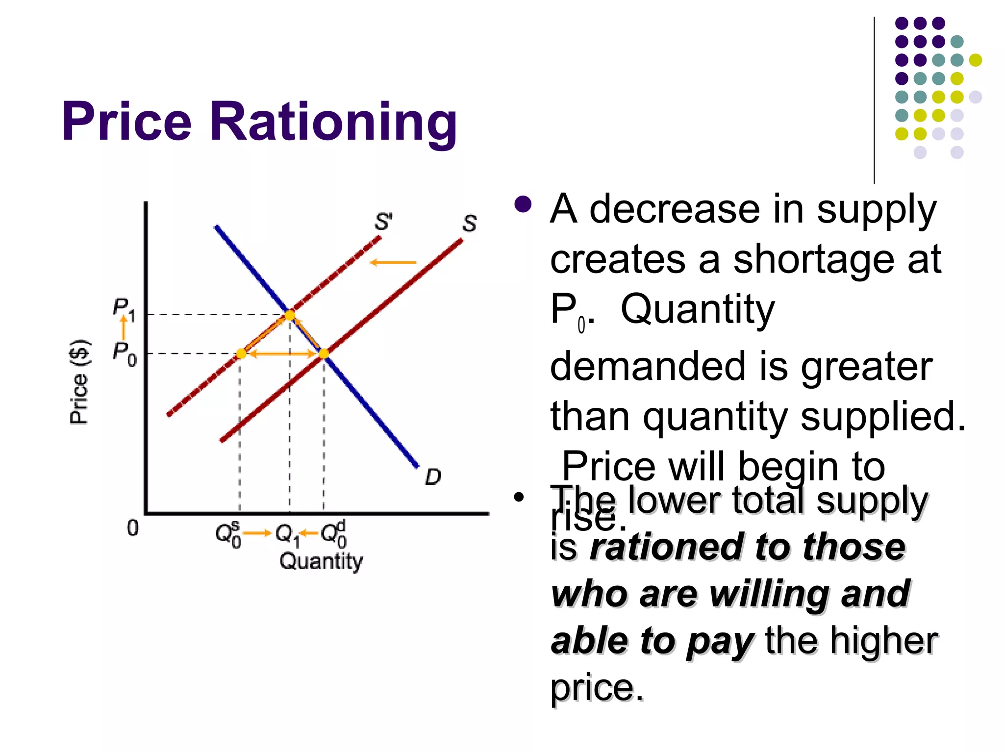
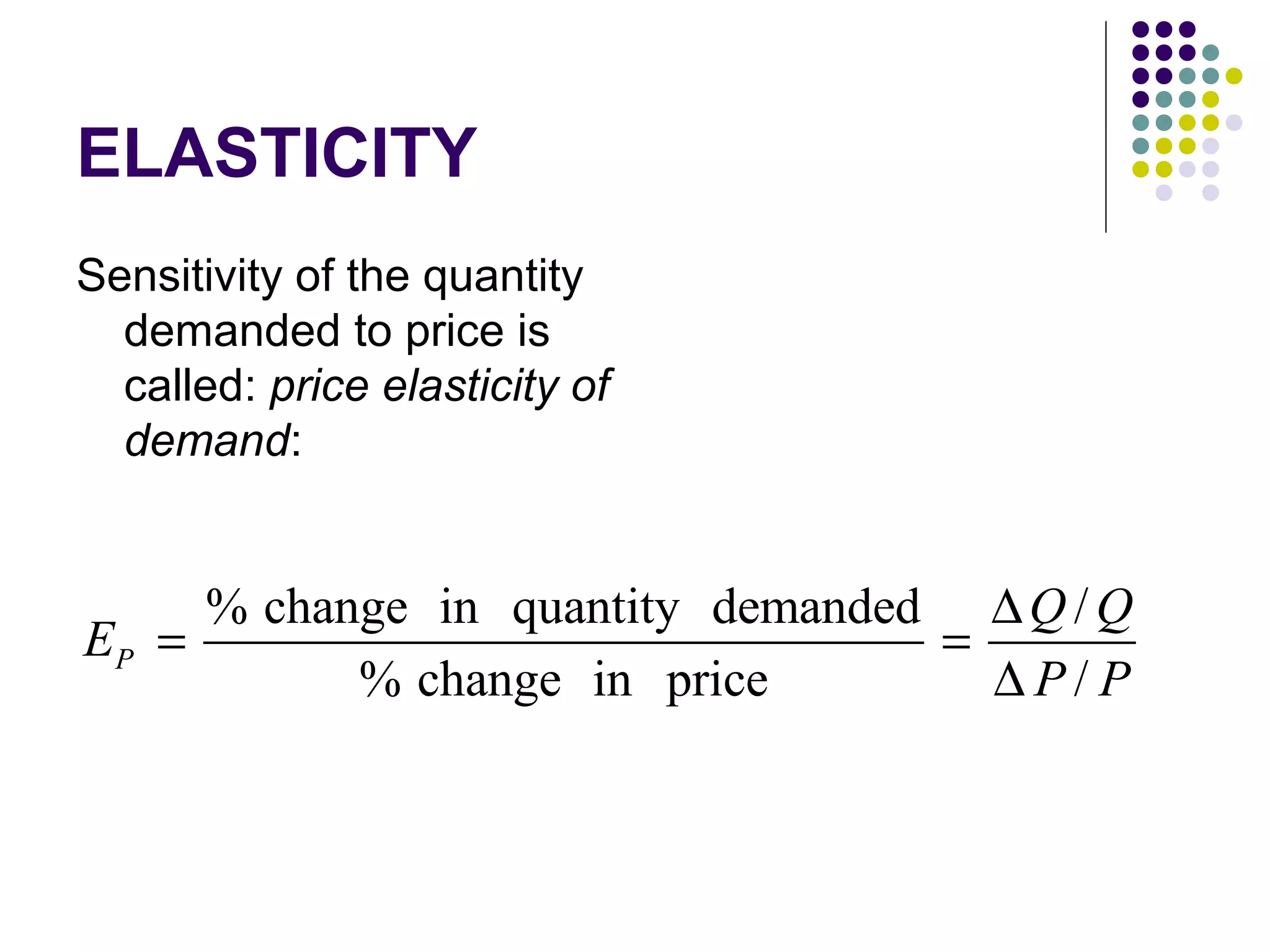
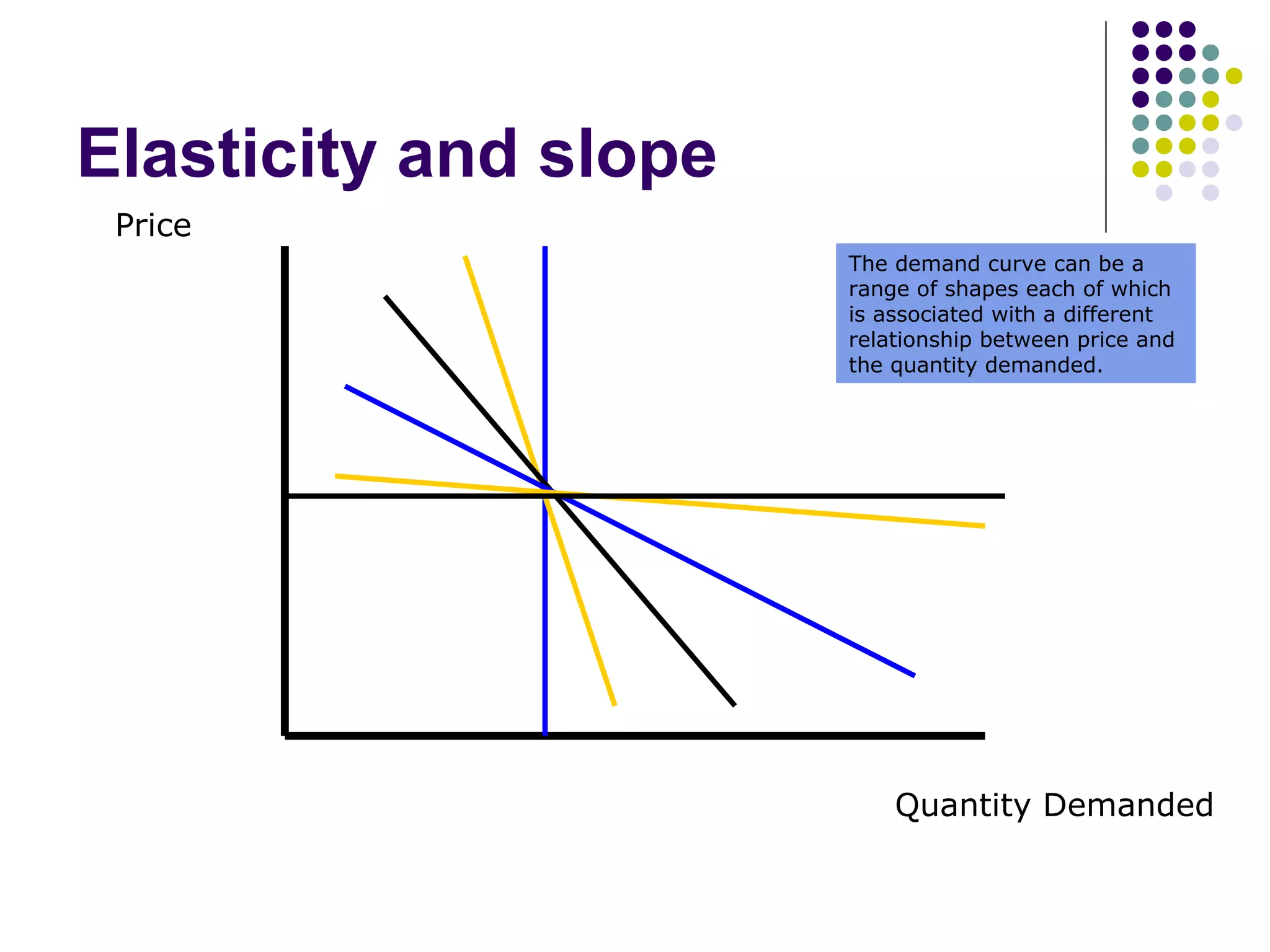
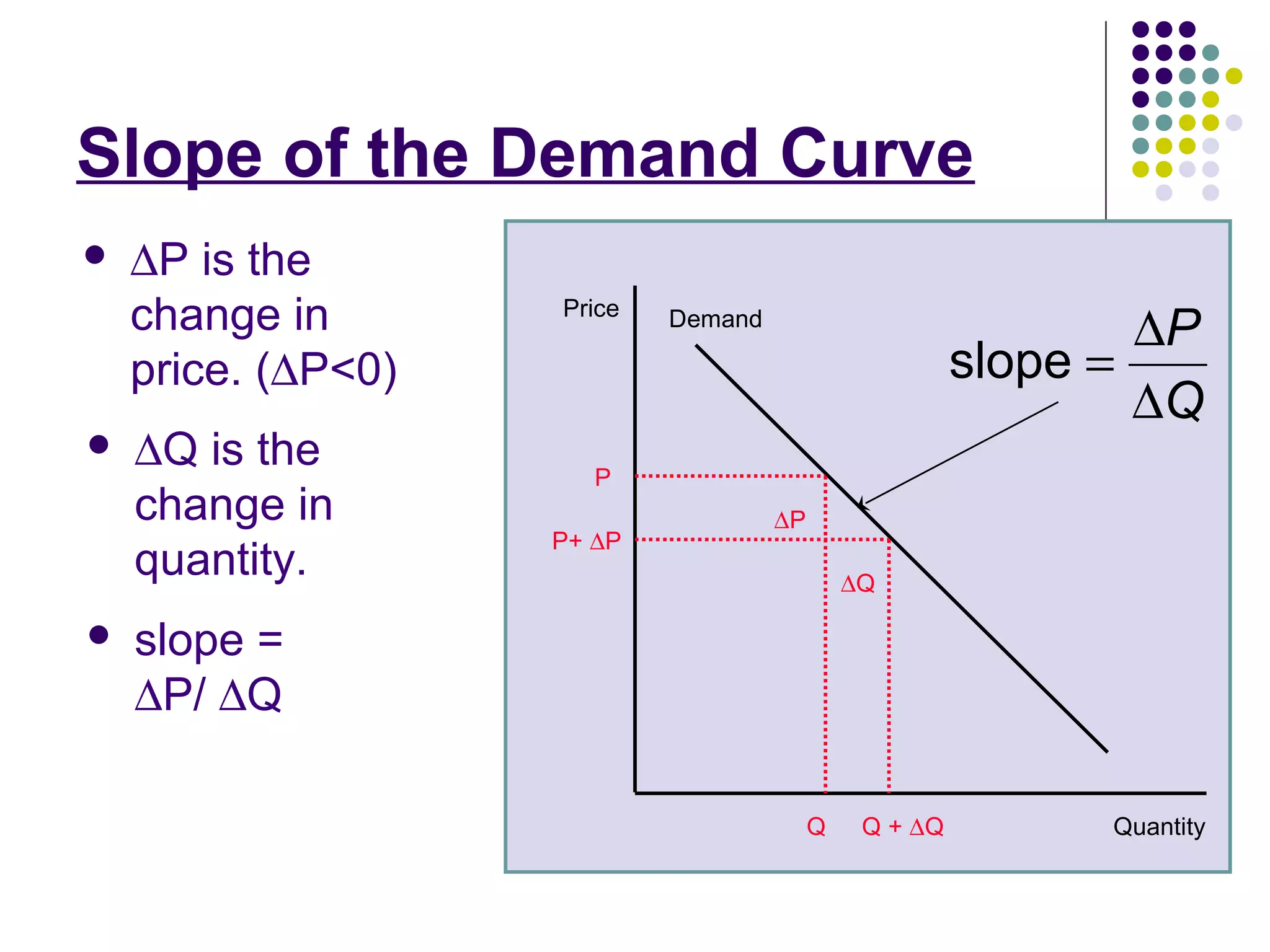
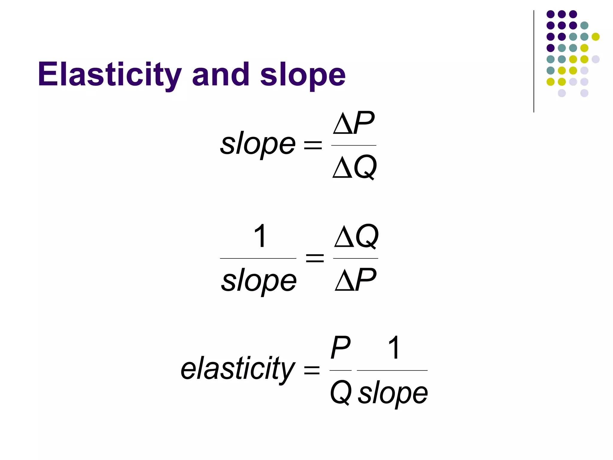
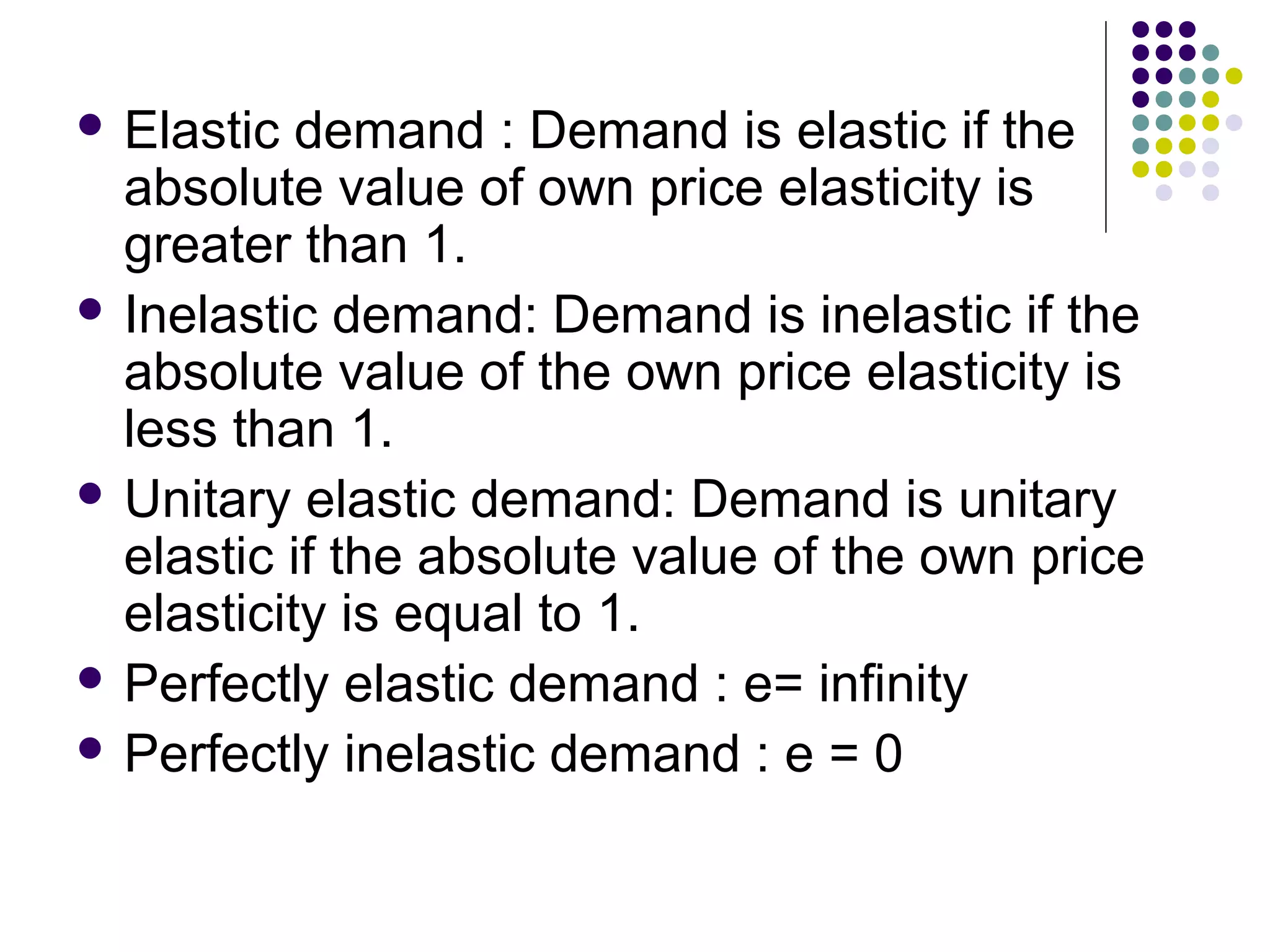
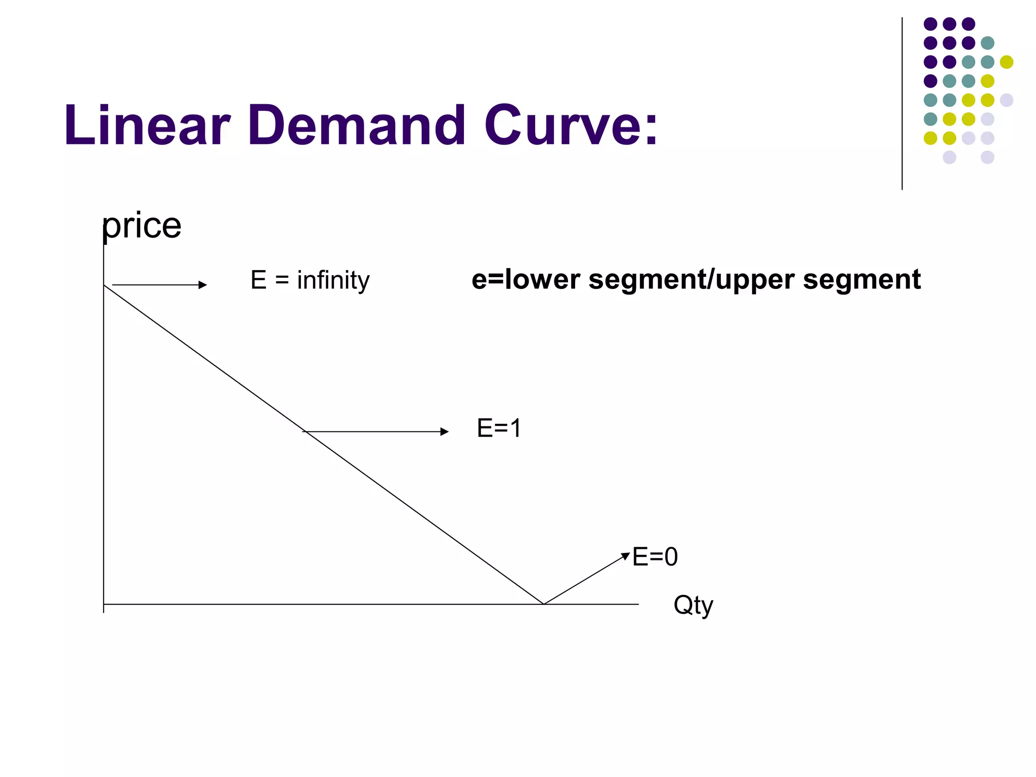
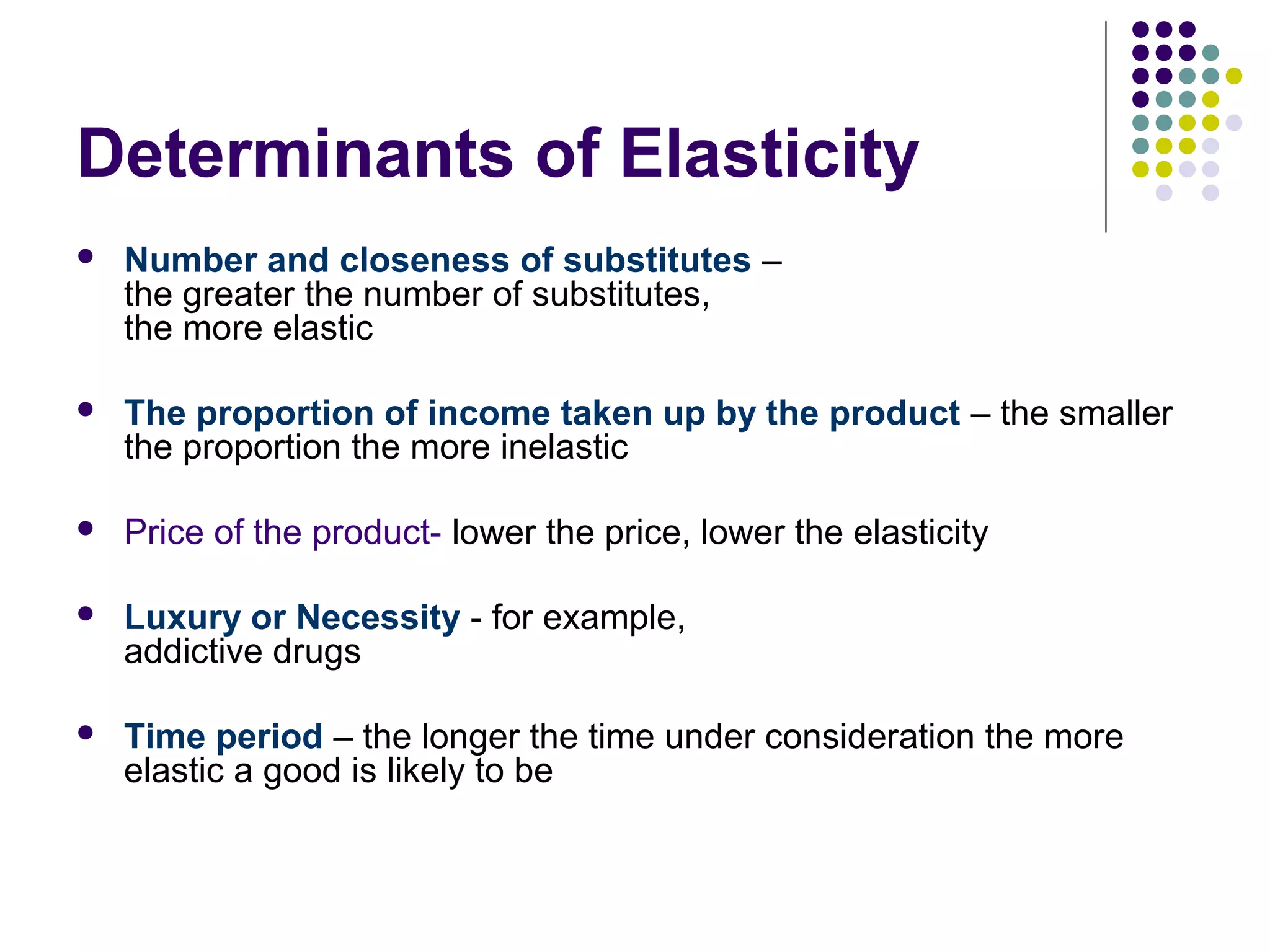
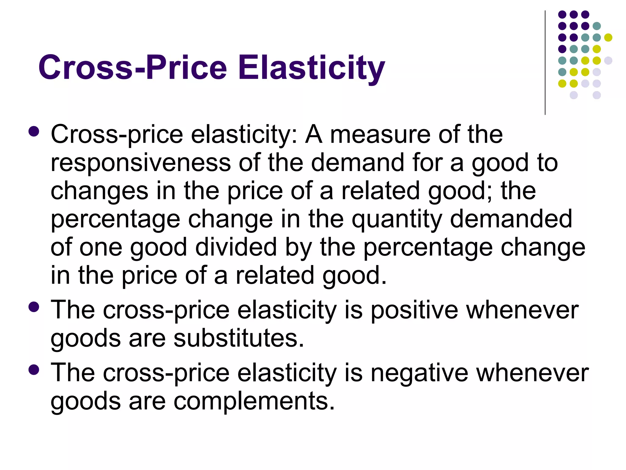
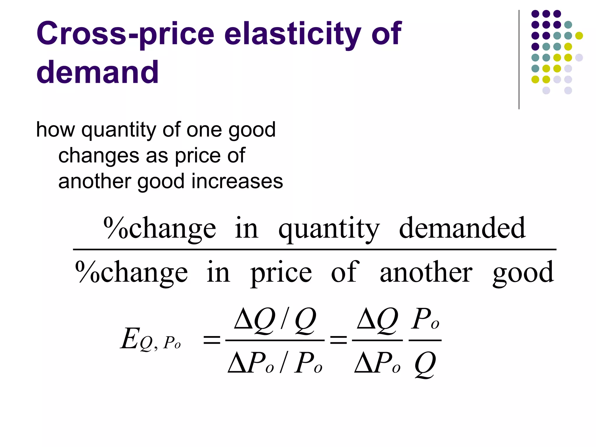
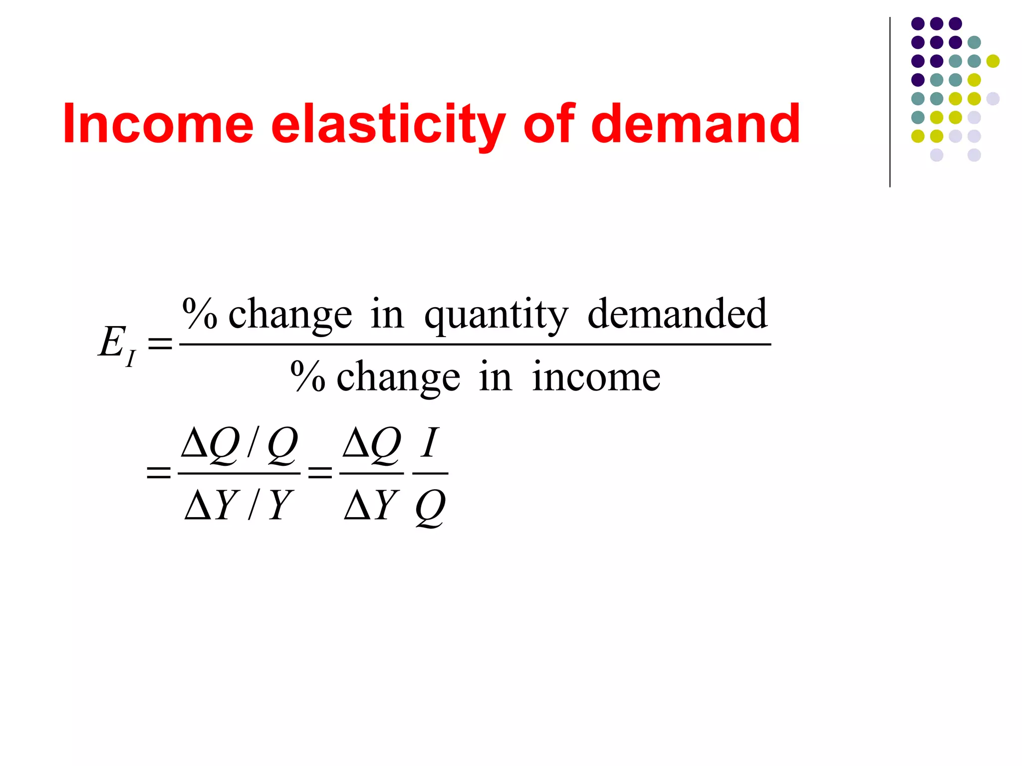
The document discusses concepts related to demand and supply, including: 1. Demand curves show the relationship between price and quantity demanded, while supply curves show the relationship between price and quantity supplied. 2. The intersection of the demand and supply curves determines the equilibrium price and quantity in a market. 3. Elasticity measures the responsiveness of demand or supply to various factors like price, income, and price of related goods. It helps to determine how demand and supply respond to changes in the market.

1. Demand and Supply
1. Demand Schedule and Demand
Curve
2. Supply Schedule and the Supply
Curve
3. Elasticity of demand and supply

2.  Demand - Total quantity customers are
willing and able to purchase.
 A demand function is a behavior function for
consumers.
 A supply function is a behavior function for
producers.
We describe market behavior using these two
functions.

3. Direct Demand and Derived
Demand
 Direct Demand-for consumption goods
Goods and services that satisfy consumer
desires.
 Derived Demand-These are sometimes
called intermediate goods.
For example, demand for steel (an
intermediate good) is derived from the
demand for final goods (e.g., automobiles).

4.  Quantity Demanded – amount of a good
that the consumer is willing to buy and able to
buy at a given price over a period of time.
 Law of Demand :All other things remaining
unchanged, the quantity demanded of a good
increases when its price decreases and vice
versa.
 This relationship can be shown by a demand
schedule, a demand curve or a demand
function.

5. Demand Schedule
 Demand Schedule
shows the different
quantities of goods that
a consumer is willing to
buy at various prices.
 Prices and quantities
normally move in
opposite directions
Prices Quantity
4 28
8 15
12 5
16 1
20 0

6. Demand Curve : A curve showing the
relationship between the price of a good and
the quantity demanded.
price
quantity

7. Demand Function:
 A demand function is a causal relationship
between a dependent variable (i.e., quantity
demanded) and various independent
variables (i.e., factors which are believed to
influence quantity demanded)
 Q = f(P)
Where Q= quantity and P = price of a good.
Example Q = 2 – 4P

8. Determinants of Demand
 Own Price
 Income of the consumer
 Price of other goods- 1. complements
2. substitutes
 Tastes and preferences
 Expectations of future prices
 Advertising
 Distribution of income

9. Types of goods
 Complementary goods are a pair of goods
consumed together. As the price of one goes
up the demand for the other falls.
Example- car and petrol
 Substitute goods are alternatives to each
other. As the price of one goes up the
demand for the other also goes up.
Example – pepsi and coke

10.  Normal goods are those goods whose
demand goes up when the consumer’s
income increases.
 Inferior goods are those goods whose
demand falls when the consumer’s income
increases.
Example : autotravel, kerosene
 Giffen goods are those goods whose demand
moves in same direction as price
 Snob or Veblen goods are those goods
whose demand falls when price falls

11. Shift of the Demand Curve
 A change in demand is reflected by shift of
the Demand curve and is caused by a
change in any of the non price determinants
of demand
price
qty
Here, the curve shifts due to an
increase in income or an
increase in price of a substitute
good etc

12.  A change in quantity demanded is however
reflected in a movement along the demand
curve and is called an extension or
contraction in demand.
 The movement from A to B is due to the
change in price of the good all other factors
remaining unchanged
A
B

13. Supply
 The quantity supplied is the number of units
that sellers want to sell over a specified
period of time at a particular price.
 Law of Supply states that all other factors
remaining unchanged the supply of a good
increases as its price increases. This can be
shown by a supply schedule, a supply curve
or a supply function.

14.  Supply schedule
 There exists a positive
relation between
quantity and price
price quantity
1 2
5 10
8 15
13 25
20 35

15.  Supply Curve:
qty
price
• Supply function shows the relation between quantity
and price.
It is a positive relation. Example : q= 4+3p

16. Determinants Of Supply
 Price
 Cost of production
 Technological progress
 Prices of related outputs
 Govt policy
All factors other than price cause a shift of the
supply curve and is called a change in supply

17. EQUILIBRIUM
 Equilibrium - perfect balance in supply and
demand
 Determines market output and price
eqm
p
q
s
dem
p

18. Market forces drive market to
equilibrium
 at prices < equilibrium level: excess demand
(amount by which quantity demanded
exceeds quantity supplied at the specified
price)
 at price > equilibrium level: excess supply
 equilibrium price is market clearing price: no
excess demand or excess supply

19. Equilibrium in a Market
Demand Price Supply
800 $3,000 2,900
1,150 $2,500 2,550
1,500 $2,000 2,200
1,850 $1,500 1,850
2,200 $1,000 1,500
2,550 $500 1,150
2,900 $0 0

20. Surplus and Shortage
 Any price above the equilibrium causes an excess
supply and any price below the equilibrium causes a
shortage.
 The market if uncontrolled will automatically arrive at
the equilibrium price at which supply equals
demand.
 Any shift in demand and supply curves will result in
a new equilibrium
 Comparison of equilibrium is called comparative
-statics

21. Price Rationing
 A decrease in supply
creates a shortage at
P0. Quantity
demanded is greater
than quantity supplied.
Price will begin to
• TrTishheee . lloowweerr ttoottaall ssuuppppllyy
iiss rraattiioonneedd ttoo tthhoossee
wwhhoo aarree wwiilllliinngg aanndd
aabbllee ttoo ppaayy tthhee hhiigghheerr
pprriiccee..

22. Alternative Price- Control
Mechanisms
• A pprriiccee cceeiilliinngg is a maximum price
that sellers may charge for a good,
usually set by government.
• Example: rent control
• AA pprriiccee fflloooorr iiss aa pprriiccee aabboovvee
eeqquuiilliibbrriiuumm pprriiccee tthhaatt tthhee bbuuyyeerrss hhaavvee
ttoo ppaayy..
• EExxaammppllee :: aaggrriiccuullttuurraall ssuuppppoorrtt pprriiccee,,
mmiinniimmuumm wwaaggeess

23. Elasticity
 Elasticity: A measure of the
responsiveness of one variable to changes
in another variable; the percentage change
in one variable that arises due to a given
percentage change in another variable.
 By converting each of these changes into
percentages, the elasticity measure does
not depend on the units in which we
measure the variables.

24. ELASTICITY
Sensitivity of the quantity
demanded to price is
called: price elasticity of
demand:
E % change in quantity demanded Q /
Q
P % change in price /
P P
= = D
D

25. Arc Elasticity
To get the average elasticity
between two points on a demand
curve we take the average of the two
end points (for both price and
quantity) and use it as the initial
value:
q2-q1/(q2+q1)/2
p2-p1/(p2+p1)/2

26. Own Price Elasticity of
Demand
 Own price elasticity: A measure of the
responsiveness of the quantity demanded of a
good to a change in the price of that good; the
percentage change in quantity demanded
divided by the percentage change in the price
of the good.
 Elastic demand: Demand is elastic if the
absolute value of the own price elasticity is
greater than 1.

27. Types of elasticities
 elastic: the quantity demanded changes more
than in proportion to a change in price
 inelastic: the quantity demanded changes
less than in proportion to a change in price

28. Elasticity and slope
Price
The demand curve can be a
range of shapes each of which
is associated with a different
relationship between price and
the quantity demanded.
Quantity Demanded

29. Slope of the Demand Curve
 DP is the
change in
Price
price. (DP<0)
P
D
slope = D
Quantity
Demand
DQ
Q Q + DQ
P
P+ DP
DP
 DQ is the
change in
quantity.
 slope =
DP/ DQ
Q

30. Elasticity and slope
slope P
= D
D
Q
1
slope
Q
P
= D
D
= 1
elasticity P
Qslope

31.  Elastic demand : Demand is elastic if the
absolute value of own price elasticity is
greater than 1.
 Inelastic demand: Demand is inelastic if the
absolute value of the own price elasticity is
less than 1.
 Unitary elastic demand: Demand is unitary
elastic if the absolute value of the own price
elasticity is equal to 1.
 Perfectly elastic demand : e= infinity
 Perfectly inelastic demand : e = 0

32. Linear Demand Curve:
price
E = infinity e=lower segment/upper segment
E=0
Qty
E=1

33. Determinants of Elasticity
 Number and closeness of substitutes –
the greater the number of substitutes,
the more elastic
 The proportion of income taken up by the product – the smaller
the proportion the more inelastic
 Price of the product- lower the price, lower the elasticity
 Luxury or Necessity - for example,
addictive drugs
 Time period – the longer the time under consideration the more
elastic a good is likely to be

34. Cross-Price Elasticity
 Cross-price elasticity: A measure of the
responsiveness of the demand for a good to
changes in the price of a related good; the
percentage change in the quantity demanded
of one good divided by the percentage change
in the price of a related good.
 The cross-price elasticity is positive whenever
goods are substitutes.
 The cross-price elasticity is negative whenever
goods are complements.

35. Cross-price elasticity of
demand
how quantity of one good
changes as price of
another good increases
%change in quantity demanded
%change in price of another good
E Q Q Q P
,
= D = D
D D
/
/ o
o
Q P
P o P o P o
Q

36. Income elasticity of demand
% change in quantity demanded
% change in income
/
/
I E
Q Q Q I
Y Y Y Q
=
= D = D
D D

37. Income Elasticity
 Income elasticity: A measure of the
responsiveness of the demand for a good to
changes in consumer income; the percentage
change in quantity demanded divided by the
percentage change in income.
 The income elasticity is positive whenever the
good is a normal good.
 The income elasticity is negative whenever the
good is an inferior good.

38. Factors affecting Income elasticity:
 Nature of the good:
 inferior goods have negative income elasticity
 Normal goods have positive income elasticity
 Luxury goods have income elasticity greater
than one
 Necessary goods have income elasticity less
than one

39. Advertising Elasticity
 The own advertising elasticity of demand for
good X defines the percentage change in the
consumption of X that results from a given
percentage change in advertising spent on X.

40. Elasticity and Total Revenue
 If demand is elastic, an increase (decrease)
in price will lead to a decrease (increase) in
total revenue.
 If demand is inelastic, an increase (decrease)
in price will lead to an increase (decrease) in
total revenue.
 Total revenue is maximized at the point
where demand is unitary elastic.

41. price revenue elasticity
Increases increases E< 1
increases decreases E>1
decreases decreases E<1
decreases increases E>1
Increases/
decreases
constant E=1

42. MARGINAL REVENUE
 TR = P.Q
MR = P + Q dP/dQ
= P(1 + Q/P. dP/dQ)
= P(1- 1/e)
= AR(1-1/e)
Hence if e=1, MR =0
if e =0 , MR = INFINITY
if e = infinity, MR = AR

43. MR,AR
QTY
E=1
E=infinity
MR
E=0

44. Total
revenue
qty
E = 1
Tr is
max

45. Elasticity of Supply
 Price Elasticity of Supply:
 The responsiveness of supply to changes
in price
 If es is inelastic (<1)- it will be difficult for suppliers to react
swiftly to changes in price
 If es is elastic(>1) – supply can react quickly to changes in
price
es =
%__ Δ_ _Q_u_a_n_t_it_y_ S_u_p_p_l_ie_d___
% Δ Price

46. Paradox of the Bumper harvest
When prices of food crops increase, the
demand does not increase proportionally.
 Hence the revenue earned by farmers fall.
 The Govt announces a floor price for the
farmers- agricultural price subsidy.
 This interference with prices comes at a cost
to the Govt in form of storage costs of Govt
granaries.

47. Application of elasticity:
 Incidence of taxation: Supply
after tax
supply
demand
e1 tax
eqm
pt
p1
p0